Statsvetenskapliga metoder

Statistiska metoder

Sirus Dehdari

Statsvetenskapliga institutionen, Stockholms universitet

Praktisk information

• Mitt kontor: F758 i F-byggnaden (våning 7). Min e-mail: sirus.dehdari@statsvet.su.se
• Föreläsningarna följer materialet i texten av Marcus Österman & Olle Folke (finns på Canvas)
• Varje “vecka” består av: föreläsning, Stata workshop, office hours, seminarier (förutom första veckan), totalt tre veckor
• I slutet av varje vecka ska ni lämna in veckans “written assignment”
• Ni lämnar in i grupp genom Canvas, samma grupper som under kursens första del

Written Assignment

• Inför seminarierna ska ni, inom er grupp, göra ett seriöst försök till att svara på samtliga frågor
• Samtliga gruppmedlemmar ska vara delaktiga i alla delar! Om någon i er grupp inte är delaktig, hör av er till er seminarieledare
• Inlämningen ska vara i pdf-format och får inte innehålla foton eller skärmdumpar överhuvudtaget
• Skriv gruppmedlemmarnas namn på inlämningen
• Ni får inte låta AI skriva inlämningarna åt er men använd gärna AI-verktyg för att få hjälp med hur man använder Stata
• Det är obligatorisk närvaro på seminarierna

Office hours och andra frågor

• Kom på office hours om ni har frågor om assignments eller kursmaterialet: dessa tillfällen finns för att underlätta er inlärning
• Jag har begränsad möjlighet att svara på frågor på mail, passa därför på under office hours
• Kontakta admin med frågor om t.ex. hur anmäla sig till tentan, var och när skriver man tentan, betyg i Ladok osv.
• Kontakta era respektive seminarieledare om ni har frågor om seminarierna, t.ex. missad närvaro osv.

Resurser

• På Canvas finns en exempeltenta (utan facit) för att ni ska få en uppfattning om hur tentan kommer att se ut på ett ungefär
• Det finns även ett dokument med övningar (med facit)
• Statistikhjälpen: praktiska Stata-guider inom bland annat regressionsanalys, deskriptiv statistik och datahantering, med kod och exempel att följa med i
• MSFS-kurser: en gratis interaktiv lärobok i matematik och statistik för samhällsvetare, med övningsuppgifter och direkt återkoppling i varje avsnitt
• Dessa föreläsningsanteckningar innehåller interaktiva figurer, tabeller och ekvationer
• Ser du inte dessa korrekt i Safari på iPhone? Testa att stänga av “Prevent Cross-Site Tracking” under Inställningar → Safari

Denna vecka ska vi lära oss följande

• Idag ska vi gå igenom följande:
  • Datastruktur och olika typer av variabler
  • Beskrivande statistik (centralitetsmått och mått på spridning)
  • Fördelningar
  • Statistik inferens
• Mer specifikt: vi ska betrakta exempel på datainsamling och olika typer av data
• Hur beskriver man data med hjälp av centralitetsmått och mått på spridning
• Förstå samplingfördelning och sannolikhetsfördelning
• Förstå vad vi menar med statistisk signifikans

Vad är grejen med kvantitativ analys?

• Vi vill lära oss något om en större population (t.ex. alla svenska hushåll)
• Tänk er följande scenario: ni jobbar för Landsbygds- och infrastrukturdepartementet med energifrågor
• På grund av höga energipriser vill departementet undersöka inomhustemperaturer hos svenska hushåll
• Hur undersöker vi detta?
• Vi kan knappast besöka alla svenska hushåll…

Datainsamling

• Vi kan göra en datainsamling (data collection) genom ett slumpmässigt urval (random sample)
• Vi väljer slumpmässigt ut, säg, 2000 hushåll som får besvara en enkätundersökning
• Enkätundersökningen består av frågor rörande inomhustemperaturen och hushållens svar utgör våra data
• Dessa data ger oss information om de 2000 hushållen men målet är att kunna säga något om hela populationen

Data

• Vad vi har sagt hittills:
  • Alla svenska hushåll utgör vår population
  • Vårt urval (sample) består av 2000 slumpmässigt valda hushåll
  • Våra data utgörs av information från enkätundersökningssvaren
• Antag att vi ber hushållen rapportera inomhustemperatur och besvara ett antal andra frågor om deras lägenhet/hus

Data: exempel på insamlade uppgifter

ID	Temp.	Yta	Medlemmar	Kommun	Utbildning
1	19	50	2	Järfälla	B.Sc.
2	18	81	3	Gagnef	Gymn
3	22	54	1	Hjo	Gymn
4	21	115	4	Huddinge	M.Sc.
\(\vdots\)
2000	21	180	2	Göteborg	Grundskola

Variabler, observationer, värden

• Varje rad i tabellen representerar en observation
• I vårt exempel är alltså varje hushåll en observation
• Kolumnerna representerar variabler
• Variabler beskriver ett objekt (i vårt exempel kan man se hushållens bostad som objekten)
• En variabel kan anta olika värden (values) (till skillnad från en konstant)
• Värdena kan vara numeriska eller i text

När observerar vi en variabel?

• Inom samhällsvetenskap observerar vi vanligtvis variabelvärden genom datainsamling av befintliga uppgifter
• Registerdata, data från olika arkiv, men också enkätundersökningar, experiment osv.
• Analysenheterna (unit of analysis) är t.ex. väljare, länder, politiska partier, eller företag
• Olika typer av data (klicka på en typ för att se ett exempel):

1. Tvärsnittsdata (cross-sectional data): varje individ (analysenhet) förekommer vid en tidpunkt
2. Paneldata: samma individer förekommer vid flera tidpunkter
3. Upprepad tvärsnittsdata (repeated cross-sectional data): data för flera tidpunkter men inte (nödvändigtvis) samma individer
4. Tidsserier (time-series data): data för flera tidpunkter för en enda individ

Land	År	BNP/capita (tkr)
Sverige	2020	498
Norge	2020	612
Danmark	2020	456

Land	År	BNP/capita (tkr)
Sverige	2019	486
Sverige	2020	498
Norge	2019	601
Norge	2020	612

Land	År	BNP/capita (tkr)
Sverige	2019	486
Norge	2019	601
Danmark	2020	456
Finland	2020	440

Land	År	BNP/capita (tkr)
Sverige	2017	470
Sverige	2018	478
Sverige	2019	486
Sverige	2020	498

Mätskala (Scales of measurement)

• Vi kan kategorisera variabler utifrån deras mätskala (scales of measurement):
  1. Nominal
  2. Ordinal
  3. Interval
  4. Ratio
• Nominalvariabler (eller kategorivariabler) är vanligtvis kategorier som inte går att rangordna: födelseland, yrke, partisympatier osv.
• I vårt exempel: Kommun är en nominalvariabel
• Ordinalvariabel: kategorierna går att rangordna
• I vårt exempel: utbildningsnivå är en ordinalvariabel

Mätskala: intervall/kvot

• Intervall- och kvotvariabler (interval/ratio): går att rangordna och har en tydlig skillnad mellan värdena
• Intervall: Tydlig skillnad mellan värdena men jämförelse mellan värdena är inte betydelsefullt
• Exempel på intervallvariabel: temperatur (i Celsius eller Fahrenheit), resultat på IQ-test
• Kvotvariabler har dessutom en absolut nollpunkt, vilket representerar total avsaknad av värde
• I vårt exempel: Temperatur är intervall, Storlek och Medlemmar är kvot

Beskrivande statistik

• Ok, så vi har samlat in data… vad gör vi nu?
• Kom ihåg vårt mål: vi vill säga något om populationen
• Att beskriva varje hushåll var för sig är inte särskilt användbart
• Vi kan sammanfatta data genom att beräkna beskrivande statistik (descriptive statistics)
• Vanligtvis beräknar vi mått på centralitet och spridning

Mått på centralitet

• Vi kan beskriva variablerna i våra data med ett antal mått
• Vanligt är att ta fram mått på centralitet (central tendency): beskriver vilka värden som är vanligt förekommande
  1. Typvärde (Mode)
  2. Median
  3. Medelvärde (Mean)
• Typvärde är det värde som förekommer oftast
• Användbart för nominal- och ordinalvariabler

Medelvärde och median

• Medianen separerar övre hälften från undre hälften
• Dvs. hälften av alla värden i vårt urval är större än medianvärdet, hälften är mindre än medianvärdet
• För att kunna skatta medianen måste vi veta hur våra värden är rangordnade
• Medelvärdet ger oss det genomsnittliga värdet i vårt urval
• Vi beräknar urvalets medelvärde för en variabel \(X\) med hjälp av följande formel:

\(\bar{X}\) = \(\dfrac{1}{n}\) \(\displaystyle\sum_{i=1}^n\) \(x_i\) = \(\dfrac{1}{n}\) ( \(x_1\) + \(x_2\) + \(\ldots + x_n\) )

Typvärde, medelvärdet, medianen

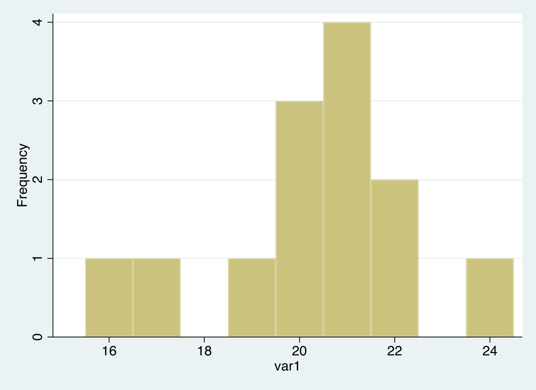
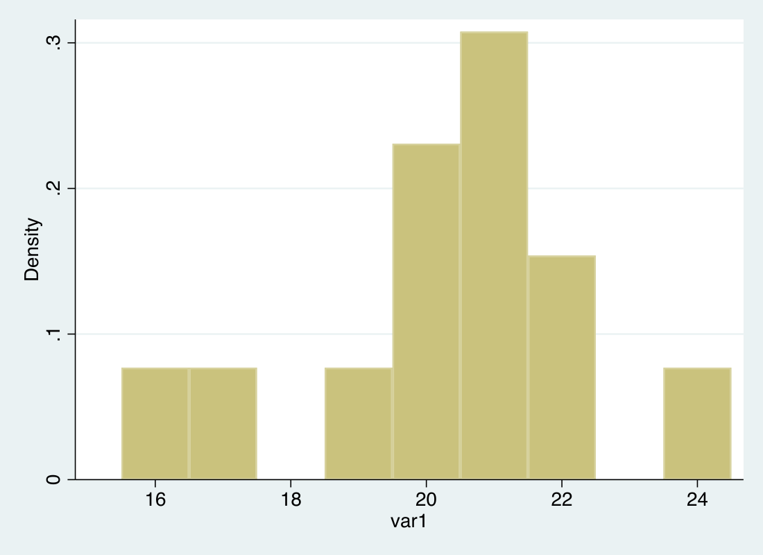
• Antag att för 13 hushåll har vi följande värden på variabeln Temperatur:

\[21, 22, 17, 19, 20, 21, 20, 21, 21, 20, 24, 22, 16\]

• Typvärdet är 21, eftersom detta värde återfinns flest gånger (fyra gånger)
• För att beräkna medianen behöver vi först rangordna värdena:

\[16, 17, 19,20,20, 20, \mathbf{21}, 21, 21, 21, 22, 22, 24\]

• Vi beräknar medelvärdet:

\[ \bar{X} = \frac{1}{13} (21+ 22+ 17+ 19+ 20+ 21+ 20+ 21+ 21+ 20+ 24+22+16) \approx 20.3 \]

Mått på spridning

• Vanligt mått på spridning är standardavvikelse (standard deviation)
• Den representerar hur värdena i våra data vanligtvis avviker från medelvärdet
• Urvalets standardavvikelse beräknas enligt följande formel:

\(s\) = \(\sqrt{\dfrac{1}{n-1}\displaystyle\sum_{i=1}^n (X_i-\bar{X})^2}\)

• Variationsbredd (range): skillnaden mellan det största och det minsta värdet i våra data
• Variationsbredd och standardavvikelse är rimliga mått enbart för intervall-/kvotvariabler

Urvalsfördelning

• Vi kan beskriva fördelningen av värdena för våra variabler med hjälp av histogram
• Dessa beskriver hur ofta förekommande (i relativa eller absoluta termer) varje värde är i våra data

• Histogram
• Data

Hushåll	Temperatur
1	21
2	22
3	17
4	19
5	20
6	21
7	20
8	21
9	21
10	20
11	24
12	22
13	16

Urvalsfördelning

• Vi kan beskriva fördelningen av värdena för våra variabler med hjälp av histogram
• Dessa beskriver hur ofta förekommande (i relativa eller absoluta termer) varje värde är i våra data

• Histogram
• Data

Hushåll	Temperatur
1	21
2	22
3	17
4	19
5	20
6	21
7	20
8	21
9	21
10	20
11	24
12	22
13	16

Populationsmedelvärde och skattningar

• Kort summering: vi vill säga något om variabeln \(X\) = inomhustemperatur hos svenska hushåll
• Populationsmedelvärde, \(\mu_X\): Genomsnittlig temperatur i populationen
• Vi använder urvalsmedelvärdet (\(\bar{X}\)) från vårt slumpmässiga urval som en skattning av populationsmedelvärdet
• Urvalsmedelvärdet från ett slumpmässigt urval är troligen inte lika med populationsmedelvärdet
• På grund av slumpen kanske vi får “överdrivet” många (översamplar) hushåll vars inomhustemperatur är högre än genomsnittet (eller lägre)

Slumpmässiga och systematiska urvalsfel

• Slumpmässiga urvalsfel: eftersom urvalet är slumpmässigt kan urvalsmedelvärdet skilja sig från populationsmedelvärdet
• Eller gör vi slumpmässiga mätfel
• Felmarginalen tar hänsyn till dessa avvikelser (mer om detta senare)
• Systematiska urvalsfel: icke-representativa urval t.ex. pga bortfall, eller systematiska mätfel
• Systematiska urvalsfel är svårare att göra något åt

Illustration: slumpmässiga och systematiska urvalsfel

100 fiktiva individer efter månadsinkomst (tkr). Klicka på en knapp för att slumpa fram ett urval på 10 — peka/klicka på en gubbe för att se dennes inkomst

function mulberry32(seed) {
  return function () {
    seed |= 0; seed = (seed + 0x6D2B79F5) | 0;
    let t = Math.imul(seed ^ (seed >>> 15), 1 | seed);
    t = (t + Math.imul(t ^ (t >>> 7), 61 | t)) ^ t;
    return ((t ^ (t >>> 14)) >>> 0) / 4294967296;
  };
}

// Fixed seed so the "population" of 100 people is identical every time
// the slide loads (not re-randomized on each render) -- so everyone in
// the room is looking at the same μ and the same 100 individuals.
// Log-normal draw: right-skewed, mimics the rough shape of Sweden's
// income distribution (most people clustered in the middle, a long
// tail of high earners). Numbers are invented, not real statistics.
// Income is kept continuous (not rounded) so incomes essentially never
// collide exactly -- rounding to whole tkr created enough duplicate
// values to force a noticeably taller, blockier swarm than the
// underlying distribution actually has.
incomePopulation = {
  const rng = mulberry32(20260813);
  const people = [];
  for (let i = 0; i < 100; i++) {
    const u1 = rng(), u2 = rng();
    const z = Math.sqrt(-2 * Math.log(u1)) * Math.cos(2 * Math.PI * u2);
    const income = Math.exp(3.33 + 0.35 * z);
    people.push({ id: i + 1, income: Math.max(12, income) });
  }
  return people;
}

incomeMu = d3.mean(incomePopulation, d => d.income)

incomePlotWidth = 1100
incomeMarginLeft = 50
incomeMarginRight = 50
incomeRowHeight = 42
incomeFigSpacing = 18
incomeTopPad = 45

incomeXScale = d3.scaleLinear()
  .domain([d3.min(incomePopulation, d => d.income) - 2, d3.max(incomePopulation, d => d.income) + 2])
  .range([incomeMarginLeft, incomePlotWidth - incomeMarginRight])

// Beeswarm-style packing: sort by income, then stack each figure into
// the first row where it doesn't overlap the previous figure already
// placed in that row -- rows fill up densely where incomes cluster,
// so the swarm's shape roughly traces the underlying distribution.
incomeLayout = {
  const sorted = [...incomePopulation].sort((a, b) => a.income - b.income);
  const rowsLastX = [];
  const placed = [];
  for (const person of sorted) {
    const x = incomeXScale(person.income);
    let row = rowsLastX.findIndex(lastX => x - lastX >= incomeFigSpacing);
    if (row === -1) {
      row = rowsLastX.length;
      rowsLastX.push(x);
    } else {
      rowsLastX[row] = x;
    }
    placed.push({ ...person, x, row });
  }
  return placed;
}

incomeWeightRichBias = (d) => d.income
incomeWeightPoorBias = (d) => 1 / d.income
incomeWeightFlat = (d) => 1

function weightedSampleWithoutReplacement(items, weightFn, n) {
  const pool = items.map(d => ({ item: d, w: weightFn(d) }));
  const chosen = [];
  for (let k = 0; k < n && pool.length > 0; k++) {
    const total = d3.sum(pool, p => p.w);
    let r = Math.random() * total;
    let idx = 0;
    for (; idx < pool.length - 1; idx++) {
      r -= pool[idx].w;
      if (r <= 0) break;
    }
    chosen.push(pool[idx].item);
    pool.splice(idx, 1);
  }
  return chosen;
}

mutable incomeSample = null

html`<div class="sd-buttons-wrap"><div class="sd-buttons">
  ${Inputs.button("🎲 Helt slumpmässigt urval", {
    value: null,
    reduce: () => {
      const sample = weightedSampleWithoutReplacement(incomePopulation, incomeWeightFlat, 10);
      mutable incomeSample = { ids: new Set(sample.map(d => d.id)), xbar: d3.mean(sample, d => d.income), method: "Helt slumpmässigt urval" };
      return null;
    }
  })}
  ${Inputs.button("⬆️ Undersamplar fattiga", {
    value: null,
    reduce: () => {
      const sample = weightedSampleWithoutReplacement(incomePopulation, incomeWeightRichBias, 10);
      mutable incomeSample = { ids: new Set(sample.map(d => d.id)), xbar: d3.mean(sample, d => d.income), method: "Undersamplar fattiga (rika oftare valda)" };
      return null;
    }
  })}
  ${Inputs.button("⬇️ Undersamplar rika", {
    value: null,
    reduce: () => {
      const sample = weightedSampleWithoutReplacement(incomePopulation, incomeWeightPoorBias, 10);
      mutable incomeSample = { ids: new Set(sample.map(d => d.id)), xbar: d3.mean(sample, d => d.income), method: "Undersamplar rika (fattiga oftare valda)" };
      return null;
    }
  })}
  ${Inputs.button("↺", {
    value: null,
    reduce: () => { mutable incomeSample = null; return null; }
  })}
</div></div>`

// Whole SVG is rebuilt on every click (cheap at n=100) -- only the
// hover/click tooltip is kept out of the reactive graph (plain D3
// show/hide via closures), so hovering never triggers a rebuild. Once
// a figure is clicked (pinned), further hovering is ignored entirely
// until the user clicks empty space to unpin -- same locked-selection
// pattern used for the household dots on L2.
//
// Each figure gets its own invisible, generously-sized hit-circle
// (radius 17, well beyond the visible stick-figure's own thin lines)
// that pointer/click handlers are attached to instead of the visible
// shapes themselves -- otherwise the actual clickable area is only the
// handful of pixels covered by 2px-wide strokes, which is what made
// pointing feel overly sensitive before.
incomeSvgWrap = {
  const maxRow = d3.max(incomeLayout, d => d.row);
  const baseY = incomeTopPad + (maxRow + 1) * incomeRowHeight;
  const axisY = baseY + 10;
  const height = axisY + 32;

  const outer = d3.create("div").attr("class", "income-pop-wrap");
  const svg = outer.append("svg")
    .attr("viewBox", `0 0 ${incomePlotWidth} ${height}`)
    .attr("width", incomePlotWidth)
    .attr("height", height)
    .attr("class", "income-pop-svg");
  const tip = outer.append("div").attr("class", "income-tip").style("display", "none");

  let pinned = false;
  function showTip(node, text) {
    tip.text(text).style("display", "block");
    const wrapRect = outer.node().getBoundingClientRect();
    const nodeRect = node.getBoundingClientRect();
    const tipNode = tip.node();
    let left = (nodeRect.left - wrapRect.left) + nodeRect.width / 2 - tipNode.offsetWidth / 2;
    let top = (nodeRect.top - wrapRect.top) - tipNode.offsetHeight - 8;
    if (left < 0) left = 0;
    if (left + tipNode.offsetWidth > wrapRect.width) left = wrapRect.width - tipNode.offsetWidth;
    if (top < 0) top = (nodeRect.bottom - wrapRect.top) + 8;
    tip.style("left", `${left}px`).style("top", `${top}px`);
  }
  function hideTip() { if (!pinned) tip.style("display", "none"); }

  // Axis line + hand-drawn ticks (short mark rising from the baseline,
  // number beneath it), matching the convention used for every other
  // number-line plot in this deck.
  svg.append("line")
    .attr("x1", incomeMarginLeft).attr("x2", incomePlotWidth - incomeMarginRight)
    .attr("y1", axisY).attr("y2", axisY).attr("stroke", "#333").attr("stroke-width", 1);
  incomeXScale.ticks(10).forEach(t => {
    svg.append("line")
      .attr("x1", incomeXScale(t)).attr("x2", incomeXScale(t))
      .attr("y1", axisY).attr("y2", axisY + 5)
      .attr("stroke", "#333").attr("stroke-width", 1);
    svg.append("text")
      .attr("x", incomeXScale(t)).attr("y", axisY + 19)
      .attr("text-anchor", "middle").attr("font-size", 14).attr("fill", "#555")
      .text(t);
  });

  const muX = incomeXScale(incomeMu);
  svg.append("line")
    .attr("x1", muX).attr("x2", muX).attr("y1", 16).attr("y2", axisY)
    .attr("stroke", "#000").attr("stroke-width", 2.5).attr("stroke-dasharray", "7,4");
  svg.append("text")
    .attr("x", muX).attr("y", 13)
    .attr("text-anchor", "middle").attr("font-size", 17).attr("fill", "#000")
    .text(`μ = ${svNum(incomeMu, 1)}`);

  if (incomeSample) {
    const xbarX = incomeXScale(incomeSample.xbar);
    svg.append("line")
      .attr("x1", xbarX).attr("x2", xbarX).attr("y1", 16).attr("y2", axisY)
      .attr("stroke", "#dc2626").attr("stroke-width", 2.5);
    svg.append("text")
      .attr("x", xbarX).attr("y", height - 4)
      .attr("text-anchor", "middle").attr("font-size", 17).attr("fill", "#dc2626")
      .text(`X̄ = ${svNum(incomeSample.xbar, 1)}`);
  }

  // Legend
  svg.append("circle").attr("cx", incomePlotWidth - 110).attr("cy", 16).attr("r", 6).attr("fill", "#dc2626");
  svg.append("text").attr("x", incomePlotWidth - 98).attr("y", 21)
    .attr("font-size", 14).attr("fill", "#333").text("= i urvalet");

  incomeLayout.forEach(d => {
    const g = svg.append("g")
      .attr("transform", `translate(${d.x}, ${baseY - d.row * incomeRowHeight})`)
      .style("cursor", "pointer");

    const sampled = incomeSample && incomeSample.ids.has(d.id);
    const color = sampled ? "#dc2626" : "#475569";

    // Soft halo behind sampled figures, in addition to the color swap
    // above -- makes the highlighted individuals unmistakable even from
    // the back of a lecture hall.
    if (sampled) {
      g.append("circle").attr("cy", -11).attr("r", 19).attr("fill", "rgba(220, 38, 38, 0.18)");
    }

    g.append("circle").attr("cy", -25).attr("r", 5).attr("fill", color);
    g.append("line").attr("x1", 0).attr("y1", -20).attr("x2", 0).attr("y2", -4).attr("stroke", color).attr("stroke-width", sampled ? 3 : 2);
    g.append("line").attr("x1", -6).attr("y1", -14).attr("x2", 6).attr("y2", -14).attr("stroke", color).attr("stroke-width", sampled ? 3 : 2);
    g.append("line").attr("x1", 0).attr("y1", -4).attr("x2", -6).attr("y2", 8).attr("stroke", color).attr("stroke-width", sampled ? 3 : 2);
    g.append("line").attr("x1", 0).attr("y1", -4).attr("x2", 6).attr("y2", 8).attr("stroke", color).attr("stroke-width", sampled ? 3 : 2);

    // Invisible, generously-sized hit target -- the actual pointer/click
    // handlers live here, not on the thin visible strokes above.
    const hit = g.append("circle")
      .attr("cy", -11).attr("r", 17)
      .attr("fill", "transparent")
      .style("pointer-events", "all");

    hit.on("pointerenter", (event) => {
      if (event.pointerType === "touch" || pinned) return;
      showTip(hit.node(), `Individ #${d.id}: ${svNum(d.income, 0)} tkr/månad`);
    })
    .on("pointerleave", (event) => {
      if (event.pointerType === "touch") return;
      hideTip();
    })
    .on("click", (event) => {
      pinned = true;
      showTip(hit.node(), `Individ #${d.id}: ${svNum(d.income, 0)} tkr/månad`);
      event.stopPropagation();
    });
  });

  svg.on("click", () => { pinned = false; tip.style("display", "none"); });

  return outer.node();
}

html`<div class="ojs-plot-wrap">
  ${incomeSvgWrap}
  <div class="ojs-plot-xlabel">Månadsinkomst (tkr)</div>
</div>`

html`<div class="ci-demo-note" style="min-height: 2.4em;">${
  !incomeSample
    ? md`*Klicka på en av knapparna ovan för att slumpa fram ett urval på 10 individer.*`
    : md`**${incomeSample.method}** — urvalsmedelvärdet är **X̄ = ${svNum(incomeSample.xbar, 1)}** tkr, jämfört med populationsmedelvärdet **μ = ${svNum(incomeMu, 1)}** tkr (skillnad: ${svNum(incomeSample.xbar - incomeMu, 1)} tkr).`
}</div>`

Hur säkra kan vi vara?

• Antag att vi enbart har slumpmässiga urvalsfel, därmed är urvalsmedelvärdet (vår skattning) inte nödvändigtvis lika med populationsmedelvärdet
• Exempel: vi väljer slumpmässigt ut 2000 hushåll och beräknar ett urvalsmedelvärde \(\bar{X} = 18\)
• Vår chef ber oss säga något om den genomsnittliga inomhustemperaturen bland svenska hushåll, vad ska vi svara?
• I just detta urval fick vi \(\bar{X} = 18\) så det är vår bästa “gissning” men hur säkra är vi på att populationsmedelvärdet inte är, säg 17?
• Det urvalsmedelvärde vi beräknar kan på grund av slumpen skilja sig från populationsmedelvärdet, därmed kanske \(\mu_{X} = 17\)

Ett intervall

• Tänk om vi kunde presentera ett intervall symmetriskt kring vår skattning \(\bar{X}\)?
• Vi säger att vi tror det sanna populationsmedelvärdet ligger mellan den undre resp. den övre gränsen av intervallet
• Till exempel, 18 \(\pm\) 3, det vill säga att det sanna populationsmedelvärdet är något mellan 15 (18-3 = 15) och 21 (18+3 = 21)
• Vi kan då använda intervallet till att avfärda (förkasta) påståenden om att den genomsnittliga inomshustemperaturen i populationen är ett värde utanför intervallet
• Hur avgör vi hur brett intervallet bör vara? Finns det en vetenskaplig metod?

Slumpvariabler

• För att förstå denna metod behöver vi först lära oss om följande begrepp/idéer:
  1. slumpvariabler,
  2. sannolikhetsfördelningar,
  3. urvalsmedelvärdet är en slumpvariabel,
  4. och har en känd sannolikhetsfördelning,
  5. som (approximativt) är en normalfördelning,
  6. och har egenskaper som hjälper oss bestämma intervallets bredd
• Först och främst, slumpvariabler: värdena vi observerar bestäms av slumpmässiga händelser
• Exempel: vädret imorgon kl 9; värdet på ett slumpmässigt valt kort från en kortlek
• Eller, inomhustemperaturen hos ett slumpmässigt valt hushåll som besvarar vår enkätundersökning

Slumpvariabler och sannolikheter

• För många slumpvariabler har de olika händelserna olika sannolikheter: vissa händelser är mer sannolika än andra
• Antag att vi har en slumpvariabel som mäter åldern på nästa person som kommer in i föreläsningssalen
• Är det sannolikt att en fyraåring kliver in? Eller att personen är mellan 20 och 40?
• För denna slumpvariabel är det uppenbart att vissa händelser, och därmed värden, är mer sannolika än andra

Sannolikhetsfördelning

• En sannolikhetsfördelning visar hur sannolika olika värden är att observeras (jämför med histogram)
• Arean under kurvan mellan två punkter visar sannolikheten att slumpvariabeln antar ett värde där emellan

// Log-normal, not the normal distribution -- students see the normal
// distribution formally a few slides later, so this generic example
// deliberately uses a differently-shaped (right-skewed) curve instead
// of previewing that exact shape here.
function logNormalPDF(x, mu, sigma) {
  if (x <= 0) return 0;
  return (1 / (x * sigma * Math.sqrt(2 * Math.PI))) * Math.exp(-((Math.log(x) - mu) ** 2) / (2 * sigma * sigma));
}

probMu = 3.3
probSigma = 0.5

probXDomain = [0, 100]

mutable probX = null

probPts = d3.range(probXDomain[0], probXDomain[1] + 0.1, 0.2).map(x => ({ x, y: logNormalPDF(x, probMu, probSigma) }))

// Trapezoidal-rule integration of the density from 0 to x, using the
// same fixed step as probPts so the shaded area and the printed
// probability are always consistent with each other.
function probCdfFrom0(x) {
  const step = 0.2;
  let area = 0;
  let prev = logNormalPDF(0, probMu, probSigma);
  for (let t = step; t <= x; t += step) {
    const cur = logNormalPDF(t, probMu, probSigma);
    area += (prev + cur) / 2 * step;
    prev = cur;
  }
  return area;
}

probPlotWidth = 860
probPlotHeight = 380
probMarginTop = 20
probMarginRight = 20
probMarginBottom = 40
probMarginLeft = 30
probYDomain = [-0.001, d3.max(probPts, d => d.y) * 1.15]

probMarks = {
  const m = [];
  if (probX !== null) {
    const shaded = probPts.filter(d => d.x <= probX);
    m.push(Plot.areaY(shaded, { x: "x", y: "y", fill: "#a855f7", fillOpacity: 0.35 }));
  }
  m.push(Plot.line(probPts, { x: "x", y: "y", stroke: "#2563eb", strokeWidth: 3 }));

  // Hand-drawn ticks (short mark rising from y=0, number beneath it)
  // instead of Plot's own axis, matching the convention used
  // throughout this deck.
  for (const t of d3.scaleLinear().domain(probXDomain).ticks(10)) {
    m.push(Plot.ruleX([{ x: t, y1: 0, y2: 0.0015 }], { x: "x", y1: "y1", y2: "y2", stroke: "#333", strokeWidth: 1 }));
    m.push(Plot.text([{ x: t, y: 0, label: String(t) }], { x: "x", y: "y", text: "label", dy: 14, fontSize: 13, fill: "#555" }));
  }

  if (probX !== null) {
    m.push(Plot.ruleX([{ x: probX, y1: 0, y2: logNormalPDF(probX, probMu, probSigma) }],
      { x: "x", y1: "y1", y2: "y2", stroke: "#7e22ce", strokeWidth: 2 }));
    m.push(Plot.text([{ x: probX, y: logNormalPDF(probX, probMu, probSigma), label: "x = " + svNum(probX, 1) }],
      { x: "x", y: "y", text: "label", dy: -10, fontSize: 14, fill: "#7e22ce" }));
  }
  m.push(Plot.ruleY([0], { stroke: "#333" }));
  return m;
}

// Transparent overlay rect for pointer capture: Plot's own event
// system only exposes marks directly under the cursor, not the raw
// pointer position, so a plain D3 rect layered on top (same x-scale
// and margins as the Plot figure below) reads the pointer's data-x
// value directly. A fresh class name (not .ojs-dots-overlay, which by
// convention is purely decorative and pointer-events: none) since this
// overlay is deliberately interactive.
probOverlay = {
  const xScale = d3.scaleLinear().domain(probXDomain).range([probMarginLeft, probPlotWidth - probMarginRight]);
  const svg = d3.create("svg")
    .attr("viewBox", `0 0 ${probPlotWidth} ${probPlotHeight}`)
    .attr("width", probPlotWidth)
    .attr("height", probPlotHeight)
    .attr("class", "ojs-click-overlay");

  svg.append("rect")
    .attr("x", probMarginLeft).attr("y", 0)
    .attr("width", probPlotWidth - probMarginLeft - probMarginRight)
    .attr("height", probPlotHeight)
    .attr("fill", "transparent")
    .style("cursor", "crosshair")
    .on("pointermove", (event) => {
      const [mx] = d3.pointer(event);
      mutable probX = Math.max(probXDomain[0], Math.min(probXDomain[1], xScale.invert(mx)));
    })
    .on("click", (event) => {
      const [mx] = d3.pointer(event);
      mutable probX = Math.max(probXDomain[0], Math.min(probXDomain[1], xScale.invert(mx)));
    });

  return svg.node();
}

html`<div class="ojs-plot-wrap" data-prevent-swipe>
  <div class="ojs-plot-overlay">
    ${Plot.plot({
      width: probPlotWidth,
      height: probPlotHeight,
      marginTop: probMarginTop,
      marginRight: probMarginRight,
      marginBottom: probMarginBottom,
      marginLeft: probMarginLeft,
      x: { domain: probXDomain, label: null, ticks: 0 },
      y: { domain: probYDomain, label: null, ticks: 0 },
      marks: probMarks
    })}
    ${probOverlay}
  </div>
  <div class="ojs-plot-xlabel">x</div>
</div>`

html`<div class="ci-demo-note" style="min-height: 2em;">${
  probX === null
    ? md`*Peka eller klicka under kurvan för att beräkna P(0 &lt; X &lt; x).*`
    : md`**P(0 &lt; X &lt; ${svNum(probX, 1)}) = ${svNum(probCdfFrom0(probX), 3)}**`
}</div>`

Tillbaka till vårt scenario

• Alla slumpvariabler följer en sannolikhetsfördelning
• I de flesta fallen vet vi dock inte vilket sannolikhetsfördelning det är
• Variabeln \(X\) = inomhustemperatur är en slumpvariabel: vi vet inte vilket värde vi kommer observera förrän vi slumpmässigt väljer ett hushåll
• Vi kan definiera nya slumpvariabler baserat på \(X\) med hjälp av matematiska operationer
• Exempel:
  • \(Y = X + 5\)
  • \(Z = X_1 + X_2\)
  • \(\bar{X} = (X_1 + X_2 + X_3 + X_4 + X_5)/5 \quad\) (=urvalsmedelvärdet)
• \(\bar{X}\) är alltså också en slumpvariabel — Visualisering

Urvalsmedelvärdet är en slumpvariabel

• \(\bar{X}\) är en slumpvariabel och följer därmed en sannolikhetsfördelning
• Eftersom \(\bar{X}\) beräknas genom ett urval kallas dess sannolikhetsfördelning för samplingsfördelning
• Kort sammanfattning:
  • Det finns något som heter slumpvariabler,
  • alla slumpvariabler har en sannolikhetsfördelning,
  • urvalsmedelvärdet (från ett slumpmässigt urval) är en slumpvariabel,
  • därmed följer den en sannolikhetsfördelning (vi kallar den för samplingsfördelning)
• Centrala gränsvärdessatsen: samplingsfördelningen hos urvalsmedelvärdet kan approximeras av en normalfördelning Simulering

Normalfördelning

• Normalfördelningen har ett antal önskvärda egenskaper
• Den är symmetrisk kring sitt medelvärde, \(\mu\)
• Samma sannolikhet att få ett värde som är mindre än medelvärdet \(\mu\) som att få ett värde större än medelvärdet \(\mu\)
• En normalfördelning kan helt och hållet beskrivas av två parametrar: medelvärdet \(\mu\) och standardavvikelsen \(\sigma\)
• Medelvärdet \(\mu\) bestämmer “mitten” av fördelningen medan standardavvikelsen \(\sigma\) beskriver spridningen

Normalfördelning: olika \(\mu\) och \(\sigma\)

För olika värden på medelvärdet \(\mu\) och standardavvikelsen \(\sigma\) får man olika läge och form på normalfördelningen

viewof mu = {
  const el = Inputs.range([80, 120], {value: 100, step: 1, label: "μ"});
  el.classList.add("small-slider");
  // Tells reveal.js's touch handler not to treat a drag that starts on
  // this slider as a slide-swipe -- without it, dragging the handle on
  // a touchscreen changes slides instead of moving the slider.
  el.setAttribute("data-prevent-swipe", "");
  return el;
}

viewof sigma = {
  const el = Inputs.range([5, 20], {value: 10, step: 1, label: "σ"});
  el.classList.add("small-slider");
  el.setAttribute("data-prevent-swipe", "");
  return el;
}

normalPDF = (x, mu, sigma) =>
  (1 / (sigma * Math.sqrt(2 * Math.PI))) * Math.exp(-0.5 * ((x - mu) / sigma) ** 2)

// Swedish uses a comma as the decimal separator, not a period -- use
// this instead of .toFixed() directly for any number shown to the
// student (JS's own number formatting is always period-based).
function svNum(x, decimals = 2) {
  return x.toFixed(decimals).replace(".", ",");
}

pts = d3.range(30, 170, 0.5).map(x => ({x, y: normalPDF(x, mu, sigma)}))

marksMuSigma = {
  const m = [
    Plot.line(pts, { x: "x", y: "y", stroke: "#2563eb", strokeWidth: 3 }),
    Plot.ruleX([{ x: mu, y1: 0, y2: 0.085 }], { x: "x", y1: "y1", y2: "y2", stroke: "#666", strokeDasharray: "4,3" })
  ];
  // Hand-drawn ticks (short mark rising from y=0, number beneath it)
  // instead of Plot's own axis, which put its numbers too far below
  // the line.
  for (const t of d3.scaleLinear().domain([30, 170]).ticks(8)) {
    m.push(Plot.ruleX([{ x: t, y1: 0, y2: 0.003 }], { x: "x", y1: "y1", y2: "y2", stroke: "#333", strokeWidth: 1 }));
    m.push(Plot.text([{ x: t, y: 0, label: String(t) }], { x: "x", y: "y", text: "label", dy: 16, fontSize: 14, fill: "#555" }));
  }
  m.push(Plot.ruleY([0], { stroke: "#333" }));
  return m;
}

html`<div class="ojs-plot-wrap">
  ${Plot.plot({
    width: 860,
    height: 440,
    marginBottom: 46,
    marginLeft: 50,
    style: "font-size: 15px;",
    x: {domain: [30, 170], label: null, ticks: 0},
    y: {domain: [-0.005, 0.09], label: null},
    marks: marksMuSigma
  })}
  <div class="ojs-plot-xlabel">x</div>
</div>`

Sannolikheter i normalfördelningen

• Sannolikheten att ett visst värde observeras för en slumpvariabel som följer en normalfördelning visas i grafen nedan
• Till exempel, vid 100 försök kommer ungefär 68 av dessa anta ett värde mellan \(\mu - \sigma\) och \(\mu + \sigma\)

mu1 = 100
sigma1 = 10

mutable sdLevel = 0

mutable simPoints = null

mutable numericExample = false

pts3 = d3.range(mu1 - 4 * sigma1, mu1 + 4 * sigma1, 0.1).map(x => ({ x, y: normalPDF(x, mu1, sigma1) }))

sdPlotWidth = 860
sdPlotHeight = 320
sdMarginTop = 20
sdMarginRight = 20
sdMarginBottom = 48
sdMarginLeft = 30
sdXDomain = [mu1 - 4.6 * sigma1, mu1 + 4.6 * sigma1]
sdYDomain = [-0.01, 0.06]

html`<div class="sd-buttons-wrap">
  <div class="sd-buttons-label">Visa intervall för:</div>
  <div class="sd-buttons">
    ${Inputs.button("σ", { value: null, reduce: () => { mutable sdLevel = 1; return null; } })}
    ${Inputs.button("2σ", { value: null, reduce: () => { mutable sdLevel = 2; return null; } })}
    ${Inputs.button("3σ", { value: null, reduce: () => { mutable sdLevel = 3; return null; } })}
    ${Inputs.button("🔢 Numeriskt exempel", {
      value: null,
      reduce: () => { mutable numericExample = !numericExample; return null; }
    })}
  </div>
  <div class="sd-buttons">
    ${Inputs.button("🎲 Simulera 100", {
      value: null,
      reduce: () => {
        mutable simPoints = {
          values: d3.range(100).map(() => mu1 + randNormal() * sigma1),
          delay: 20,
          duration: 900,
          radius: 4
        };
        return null;
      }
    })}
    ${Inputs.button("🎲 Simulera 1000", {
      value: null,
      reduce: () => {
        mutable simPoints = {
          values: d3.range(1000).map(() => mu1 + randNormal() * sigma1),
          delay: 3.5,
          duration: 900,
          radius: 2
        };
        return null;
      }
    })}
    ${Inputs.button("↺", {
      value: null,
      reduce: () => {
        mutable sdLevel = 0;
        mutable simPoints = null;
        return null;
      }
    })}
  </div>
</div>`

marksSd = {
  const m = [];
  const lo = mu1 - sdLevel * sigma1;
  const hi = mu1 + sdLevel * sigma1;
  if (sdLevel > 0) {
    const band = pts3.filter(d => d.x >= lo && d.x <= hi);
    m.push(Plot.areaY(band, { x: "x", y: "y", fill: "#a855f7", fillOpacity: 0.35 }));
  }
  m.push(Plot.line(pts3, { x: "x", y: "y", stroke: "#2563eb", strokeWidth: 3 }));
  m.push(Plot.ruleX([{ x: mu1, y1: 0, y2: normalPDF(mu1, mu1, sigma1) }],
    { x: "x", y1: "y1", y2: "y2", stroke: "#666", strokeDasharray: "4,3", strokeWidth: 1.5 }));
  m.push(Plot.text([{ x: mu1, y: 0, label: "μ" }], { x: "x", y: "y", text: "label", dy: 18, fontSize: 15 }));
  if (numericExample) {
    // Placed one row below the μ−σ/μ+σ numeric labels (dy: 54, not 36)
    // so it never overlaps them -- those sit close to μ on the x-axis
    // (only ±σ apart) and would collide with this label on the same
    // row. Fixed at 54 regardless of sdLevel, rather than only moving
    // down when sdLevel > 0, so this label's position never jumps
    // depending on which other button was clicked.
    m.push(Plot.text([{ x: mu1, y: 0, label: `μ = ${mu1}, σ = ${sigma1}` }],
      { x: "x", y: "y", text: "label", dy: 54, fontSize: 13, fill: "#000" }));
  }
  if (sdLevel > 0) {
    const sign = sdLevel === 1 ? "σ" : sdLevel + "σ";
    const pct = { 1: "68,27 %", 2: "95,45 %", 3: "99,73 %" }[sdLevel];
    m.push(Plot.ruleX([{ x: lo, y1: 0, y2: normalPDF(lo, mu1, sigma1) }],
      { x: "x", y1: "y1", y2: "y2", stroke: "#7e22ce", strokeWidth: 1 }));
    m.push(Plot.ruleX([{ x: hi, y1: 0, y2: normalPDF(hi, mu1, sigma1) }],
      { x: "x", y1: "y1", y2: "y2", stroke: "#7e22ce", strokeWidth: 1 }));
    m.push(Plot.text([{ x: lo, y: 0, label: "μ − " + sign }],
      { x: "x", y: "y", text: "label", dy: 18, fontSize: 14, fill: "#7e22ce" }));
    m.push(Plot.text([{ x: hi, y: 0, label: "μ + " + sign }],
      { x: "x", y: "y", text: "label", dy: 18, fontSize: 14, fill: "#7e22ce" }));
    m.push(Plot.text([{ x: mu1, y: normalPDF(mu1, mu1, sigma1), label: pct }],
      { x: "x", y: "y", text: "label", dy: -10, fontSize: 16, fill: "#7e22ce" }));
    if (numericExample) {
      const delta = sdLevel * sigma1;
      m.push(Plot.text([{ x: lo, y: 0, label: `μ − ${sign} = ${mu1} − ${delta} = ${lo}` }],
        { x: "x", y: "y", text: "label", dy: 36, fontSize: 13, fill: "#7e22ce" }));
      m.push(Plot.text([{ x: hi, y: 0, label: `μ + ${sign} = ${mu1} + ${delta} = ${hi}` }],
        { x: "x", y: "y", text: "label", dy: 36, fontSize: 13, fill: "#7e22ce" }));
    }
  }
  m.push(Plot.ruleY([0], { stroke: "#333" }));
  return m;
}

// Falling-dots overlay: built with raw D3 (not Observable Plot), using
// our own linear scale that matches the Plot figure's own domain and
// pixel margins exactly, so dots land at the right x-position on the
// axis. Kept as a *separate* SVG layered on top of the Plot figure via
// CSS, so it only depends on simPoints -- switching σ/2σ/3σ afterwards
// never re-triggers the fall animation or disturbs the dots.
dotsOverlay = {
  const xScale = d3.scaleLinear().domain(sdXDomain).range([sdMarginLeft, sdPlotWidth - sdMarginRight]);
  // The y-domain's minimum is -0.01, not 0 (there's a sliver of
  // padding below the axis), so "where y=0 sits" is NOT simply the
  // bottom margin -- it has to go through the same scale Plot itself
  // uses, otherwise the dots land below the visible axis rule.
  const yScale = d3.scaleLinear().domain(sdYDomain).range([sdPlotHeight - sdMarginBottom, sdMarginTop]);
  const svg = d3.create("svg")
    .attr("viewBox", `0 0 ${sdPlotWidth} ${sdPlotHeight}`)
    .attr("width", sdPlotWidth)
    .attr("height", sdPlotHeight)
    .attr("class", "ojs-dots-overlay");

  if (simPoints) {
    const axisY = yScale(0);
    const topY = sdMarginTop;
    svg.selectAll("circle")
      .data(simPoints.values)
      .join("circle")
      .attr("cx", d => xScale(d))
      .attr("cy", topY)
      .attr("r", simPoints.radius)
      .attr("fill", "#dc2626")
      .attr("fill-opacity", 0.7)
      .transition()
      .delay((d, i) => i * simPoints.delay)
      .duration(simPoints.duration)
      .ease(d3.easeCubicIn)
      .attr("cy", axisY);
  }

  return svg.node();
}

html`<div class="ojs-plot-wrap">
  <div class="ojs-plot-overlay">
    ${Plot.plot({
      width: sdPlotWidth,
      height: sdPlotHeight,
      marginTop: sdMarginTop,
      marginRight: sdMarginRight,
      marginBottom: sdMarginBottom,
      marginLeft: sdMarginLeft,
      x: { domain: sdXDomain, label: null, ticks: 0 },
      y: { domain: [-0.01, 0.09], label: null, ticks: 0 },
      marks: marksSd
    })}
    ${dotsOverlay}
  </div>
  <div class="ojs-plot-xlabel">x</div>
</div>`

html`<div class="ci-demo-note">${
  !simPoints
    ? ""
    : sdLevel === 0
      ? md`*Välj ett intervall (σ, 2σ eller 3σ) ovan för att se hur många av de ${simPoints.values.length} simulerade observationerna som hamnar inom det.*`
      : (() => {
          const lo = mu1 - sdLevel * sigma1, hi = mu1 + sdLevel * sigma1;
          const n = simPoints.values.length;
          const count = simPoints.values.filter(v => v >= lo && v <= hi).length;
          const sign = sdLevel === 1 ? "σ" : sdLevel + "σ";
          return md`**${count}** av ${n} simulerade observationer (**${svNum(100 * count / n, 1)} %**) hamnade inom **${sign}** från medelvärdet.`;
        })()
}</div>`

Exempel: pizzaleverans

• Antag att tiden det tar innan en beställd pizza levereras följer en normalfördelning med medelvärde \(\mu = 30\) minuter och standardavvikelse \(\sigma = 5\) minuter
• Varje knapptryckning nedan simulerar en enskild beställning: en pizza slumpas fram och “landar” på tallinjen vid sin leveranstid

muP = 30
sigmaP = 5

mutable sdLevelP = 0

mutable pizzaHistory = []

ptsP = d3.range(muP - 4.6 * sigmaP, muP + 4.6 * sigmaP, 0.1).map(x => ({ x, y: normalPDF(x, muP, sigmaP) }))

pPlotWidth = 860
pPlotHeight = 320
pMarginTop = 20
pMarginRight = 20
pMarginBottom = 40
pMarginLeft = 30
pXDomain = [muP - 4.6 * sigmaP, muP + 4.6 * sigmaP]
pYDomain = [-0.005, 0.09]
pBinWidth = 0.1

html`<div class="sd-buttons-wrap">
  <div class="sd-buttons-label">Visa intervall för:</div>
  <div class="sd-buttons">
    ${Inputs.button("σ", { value: null, reduce: () => { mutable sdLevelP = 1; return null; } })}
    ${Inputs.button("2σ", { value: null, reduce: () => { mutable sdLevelP = 2; return null; } })}
    ${Inputs.button("3σ", { value: null, reduce: () => { mutable sdLevelP = 3; return null; } })}
  </div>
  <div class="sd-buttons">
    ${Inputs.button("🍕 Beställ pizza", {
      value: null,
      reduce: () => {
        mutable pizzaHistory = [...pizzaHistory, muP + randNormal() * sigmaP];
        return null;
      }
    })}
    ${Inputs.button("↺", {
      value: null,
      reduce: () => {
        mutable sdLevelP = 0;
        mutable pizzaHistory = [];
        return null;
      }
    })}
  </div>
</div>`

marksP = {
  const m = [];
  const lo = muP - sdLevelP * sigmaP;
  const hi = muP + sdLevelP * sigmaP;
  if (sdLevelP > 0) {
    const band = ptsP.filter(d => d.x >= lo && d.x <= hi);
    m.push(Plot.areaY(band, { x: "x", y: "y", fill: "#a855f7", fillOpacity: 0.35 }));
  }
  m.push(Plot.line(ptsP, { x: "x", y: "y", stroke: "#2563eb", strokeWidth: 3 }));

  // Plot's own axis put its tick numbers too far below the number
  // line, so it's suppressed (ticks: 0 below) and drawn by hand here
  // instead: a short mark rising from y=0, number directly beneath it.
  for (const t of d3.scaleLinear().domain(pXDomain).ticks(8)) {
    m.push(Plot.ruleX([{ x: t, y1: 0, y2: 0.003 }],
      { x: "x", y1: "y1", y2: "y2", stroke: "#333", strokeWidth: 1 }));
    m.push(Plot.text([{ x: t, y: 0, label: String(t) }],
      { x: "x", y: "y", text: "label", dy: 14, fontSize: 14, fill: "#555" }));
  }

  m.push(Plot.ruleX([{ x: muP, y1: 0, y2: normalPDF(muP, muP, sigmaP) }],
    { x: "x", y1: "y1", y2: "y2", stroke: "#666", strokeDasharray: "4,3", strokeWidth: 1.5 }));
  if (sdLevelP > 0) {
    const pct = { 1: "68,27 %", 2: "95,45 %", 3: "99,73 %" }[sdLevelP];
    m.push(Plot.ruleX([{ x: lo, y1: 0, y2: normalPDF(lo, muP, sigmaP) }],
      { x: "x", y1: "y1", y2: "y2", stroke: "#7e22ce", strokeWidth: 1 }));
    m.push(Plot.ruleX([{ x: hi, y1: 0, y2: normalPDF(hi, muP, sigmaP) }],
      { x: "x", y1: "y1", y2: "y2", stroke: "#7e22ce", strokeWidth: 1 }));
    m.push(Plot.text([{ x: muP, y: normalPDF(muP, muP, sigmaP), label: pct }],
      { x: "x", y: "y", text: "label", dy: -10, fontSize: 16, fill: "#7e22ce" }));
  }
  m.push(Plot.ruleY([0], { stroke: "#333" }));
  // Hand-drawn arrowhead at the line's right end (rather than relying
  // on Plot's own x.label/labelArrow, which appends a text arrow after
  // the label and needs vertical room below the axis that this compact
  // layout doesn't have) -- a small right-pointing glyph sitting right
  // on the axis line itself.
  m.push(Plot.text([{ x: pXDomain[1], y: 0, label: "▶" }],
    { x: "x", y: "y", text: "label", dx: 5, dy: 1, fontSize: 11, fill: "#333" }));
  return m;
}

// Growing dot-histogram of past pizza deliveries: each order stacks a
// new dot on top of previous ones that landed in the same time-bin.
// Only the newest dot animates falling -- earlier ones are drawn
// directly in their already-landed stacked position, so re-ordering
// doesn't replay the whole history's animation every time.
pizzaOverlay = {
  const xScale = d3.scaleLinear().domain(pXDomain).range([pMarginLeft, pPlotWidth - pMarginRight]);
  const yScale = d3.scaleLinear().domain(pYDomain).range([pPlotHeight - pMarginBottom, pMarginTop]);
  const axisY = yScale(0);
  const dotR = 5;
  const step = 2 * dotR + 1;

  const svg = d3.create("svg")
    .attr("viewBox", `0 0 ${pPlotWidth} ${pPlotHeight}`)
    .attr("width", pPlotWidth)
    .attr("height", pPlotHeight)
    .attr("class", "ojs-dots-overlay");

  // Stack dots on the exact value, rounded to one decimal -- the same
  // precision the delivery time itself is displayed at -- rather than
  // a wider bin, so two orders only stack when they actually rounded
  // to the same tenth of a minute.
  const roundOf = v => Math.round(v / pBinWidth) * pBinWidth;
  const seenPerValue = new Map();
  const placed = pizzaHistory.map(v => {
    const r = roundOf(v).toFixed(1);
    const stackIndex = seenPerValue.get(r) ?? 0;
    seenPerValue.set(r, stackIndex + 1);
    const cx = xScale(Number(r));
    const cy = axisY - stackIndex * step - dotR;
    return { cx, cy };
  });

  svg.selectAll("circle")
    .data(placed)
    .join("circle")
    .attr("cx", d => d.cx)
    .attr("cy", (d, i) => i === placed.length - 1 ? pMarginTop : d.cy)
    .attr("r", dotR)
    .attr("fill", "#dc2626")
    .attr("fill-opacity", 0.8)
    .each(function (d, i) {
      if (i === placed.length - 1) {
        d3.select(this).transition().duration(700).ease(d3.easeCubicIn).attr("cy", d.cy);
      }
    });

  return svg.node();
}

html`<div class="ojs-plot-wrap">
  <div class="ojs-plot-overlay">
    ${Plot.plot({
      width: pPlotWidth,
      height: pPlotHeight,
      marginTop: pMarginTop,
      marginRight: pMarginRight,
      marginBottom: pMarginBottom,
      marginLeft: pMarginLeft,
      style: "font-size: 15px;",
      x: { domain: pXDomain, label: null, ticks: 0 },
      y: { domain: pYDomain, label: null, ticks: 0 },
      marks: marksP
    })}
    ${pizzaOverlay}
  </div>
  <div class="ojs-plot-xlabel">Minuter</div>
</div>`

html`<div class="ci-demo-note">${
  pizzaHistory.length === 0
    ? md`*Klicka på "Beställ pizza" för att simulera en leveranstid. Välj gärna ett intervall (σ, 2σ eller 3σ) först.*`
    : (() => {
        const n = pizzaHistory.length;
        const last = pizzaHistory[n - 1];
        const lastLine = `Din senaste pizza kom efter **${svNum(last, 1)}** minuter.`;
        if (sdLevelP === 0) return md`${lastLine} Du har beställt **${n}** ${n === 1 ? "pizza" : "pizzor"} totalt.`;
        const lo = muP - sdLevelP * sigmaP, hi = muP + sdLevelP * sigmaP;
        const count = pizzaHistory.filter(v => v >= lo && v <= hi).length;
        const sign = sdLevelP === 1 ? "σ" : sdLevelP + "σ";
        return md`${lastLine} Du har beställt **${n}** ${n === 1 ? "pizza" : "pizzor"} totalt, varav **${count}** (**${svNum(100 * count / n, 1)} %**) anlände inom **${sign}** från medelvärdet.`;
      })()
}</div>`

\(\bar{X}\) följer (typ) en normalfördelning

• Igen: Centrala gränsvärdessatsen visar att urvalsmedelvärdet följer (typ) en normalfördelning (egentligen \(t\)-fördelning, Läs mer)
• Dessutom vet vi att \(\bar{X}\) för slumpvariabeln \(X\) beräknat med vårt urval kommer från en normalfördelning som har ett \(\mu\) som är lika med populationsmedelvärdet för \(X\)
• Men vi vet inte värdena för \(\mu\) eller \(\sigma\) (kallas för standardfel i en samplingsfördelning)
• Vi vet dock att ungefär 95 procent av alla möjliga slumpmässiga urval kommer ge ett urvalsmedelvärde inom intervallet \(\mu - 2 \times \sigma\) och \(\mu + 2 \times \sigma\)

Konfidensintervall

• Vi vet att, drar vi 100 slumpmässiga urval kommer 95 av dessa ge oss ett urvalsmedelvärde \(\bar{X}\) inom intervallet \(\mu - 2 \times \sigma\) och \(\mu + 2 \times \sigma\) (symmetriskt kring \(\mu\))
• Vi vet dock inte värdet på \(\sigma\); men tänk om vi kan skatta det?
• Då vet vi “bredden” på intervallet kring medelvärdet \(\mu\) som täcker 95 av 100 av urvalsmedelvärdena
• Kom ihåg målet: presentera en skattning av populationsmedelvärdet tillsammans med ett intervall av möjliga värden
• Om det \(\bar{X}\) vi beräknar finns inom det intervallet kring \(\mu\), så måste också \(\mu\) finnas inom ett liknande intervall kring vårt \(\bar{X}\)

Täcker intervallet \(\mu\)?

Det skuggade området täcker \(\mu \pm 2\sigma\), det vill säga 95,45 % av alla realiseringar av \(\bar{X}\) som hamnar närmast \(\mu\). Slumpa fram ett urvalsmedelvärde \(\bar{X}\) för att se om ett lika brett intervall kring \(\bar{X}\) täcker \(\mu\)

mu0 = 20
sigma0 = 2

function randNormal() {
  const u1 = Math.random(), u2 = Math.random();
  return Math.sqrt(-2 * Math.log(u1)) * Math.cos(2 * Math.PI * u2);
}

mutable draw = null

html`<div class="dice-rows">
  ${Inputs.button("🎲", {
    value: null,
    reduce: () => {
      let z;
      do { z = randNormal(); } while (Math.abs(z) >= 2);
      mutable draw = { x: mu0 + z * sigma0, inside: true };
      return null;
    }
  })}
  <span>Slumpa en realisering: <strong>inom</strong> 95 %-intervallet</span>
  ${Inputs.button("🎲", {
    value: null,
    reduce: () => {
      let z;
      do { z = randNormal(); } while (Math.abs(z) < 2);
      mutable draw = { x: mu0 + z * sigma0, inside: false };
      return null;
    }
  })}
  <span>Slumpa en realisering: <strong>utanför</strong> 95 %-intervallet</span>
  ${Inputs.button("🎲", {
    value: null,
    reduce: () => {
      const z = randNormal();
      mutable draw = { x: mu0 + z * sigma0, inside: Math.abs(z) < 2 };
      return null;
    }
  })}
  <span>Slumpa en realisering: helt fritt</span>
  ${Inputs.button("↺", {
    value: null,
    reduce: () => {
      mutable draw = null;
      return null;
    }
  })}
  <span>Ta bort realiseringen (börja om)</span>
</div>`

pts2 = d3.range(mu0 - 4 * sigma0, mu0 + 4 * sigma0, 0.05)
  .map(x => ({ x, y: normalPDF(x, mu0, sigma0) }))

marks = {
  const m = [];
  const bandPts = pts2.filter(d => d.x >= mu0 - 2 * sigma0 && d.x <= mu0 + 2 * sigma0);
  m.push(Plot.areaY(bandPts, { x: "x", y: "y", fill: "#a855f7", fillOpacity: 0.35 }));
  m.push(Plot.line(pts2, { x: "x", y: "y", stroke: "#2563eb", strokeWidth: 3 }));
  m.push(Plot.ruleX([{ x: mu0, y1: 0, y2: 0.22 }], { x: "x", y1: "y1", y2: "y2", stroke: "#000", strokeWidth: 2, strokeDasharray: "6,4" }));

  // Hand-drawn ticks (short mark rising from y=0, number beneath it)
  // instead of Plot's own axis, which put its numbers too far below
  // the line.
  for (const t of d3.scaleLinear().domain([mu0 - 4 * sigma0, mu0 + 4 * sigma0]).ticks(8)) {
    m.push(Plot.ruleX([{ x: t, y1: 0, y2: 0.008 }], { x: "x", y1: "y1", y2: "y2", stroke: "#333", strokeWidth: 1 }));
    m.push(Plot.text([{ x: t, y: 0, label: String(t) }], { x: "x", y: "y", text: "label", dy: 14, fontSize: 11, fill: "#555" }));
  }

  m.push(Plot.text([{ x: mu0, y: 0, label: "μ = 20" }], { x: "x", y: "y", text: "label", dy: 32, fontSize: 13, fill: "#000" }));
  if (draw) {
    const col = draw.inside ? "#dc2626" : "#f59e0b";
    m.push(Plot.link([{ x1: draw.x - 2 * sigma0, x2: draw.x + 2 * sigma0, y1: 0.06, y2: 0.06 }],
      { x1: "x1", x2: "x2", y1: "y1", y2: "y2", stroke: col, strokeWidth: 4 }));
    m.push(Plot.ruleX([{ x: draw.x, y1: 0, y2: 0.06 }],
      { x: "x", y1: "y1", y2: "y2", stroke: col, strokeWidth: 1 }));
    m.push(Plot.dot([{ x: draw.x, y: 0 }], { x: "x", y: "y", r: 6, fill: col }));
    m.push(Plot.text([{ x: draw.x, y: 0.06, label: "X̄ = " + svNum(draw.x, 2) }],
      { x: "x", y: "y", text: "label", dy: -10, fontSize: 15, fill: col }));
  }
  m.push(Plot.ruleY([0], { stroke: "#333" }));
  return m;
}

html`<div class="ojs-plot-row">
  <div class="ojs-plot-wrap">
    ${Plot.plot({
      width: 620,
      height: 300,
      marginBottom: 52,
      marginLeft: 50,
      x: { domain: [mu0 - 4 * sigma0, mu0 + 4 * sigma0], label: null, ticks: 0 },
      y: { domain: [-0.02, 0.24], label: null, ticks: 0 },
      marks: marks
    })}
    <div class="ojs-plot-xlabel">x</div>
  </div>
  <div class="ojs-plot-caption">
    95 %-intervall<br>
    [μ − 2σ, μ + 2σ]<br>
    = [${mu0 - 2 * sigma0}, ${mu0 + 2 * sigma0}]
  </div>
</div>`

html`<div class="ci-demo-note">${
  draw
    ? (() => {
        const lo = svNum(draw.x - 2 * sigma0, 2), hi = svNum(draw.x + 2 * sigma0, 2);
        return draw.inside
          ? md`✅ Detta X̄ (= ${svNum(draw.x, 2)}) är en av de **95,45 %** av realiseringarna som hamnar inom 2σ från μ. Ett lika brett intervall, dvs [${lo}, ${hi}], kring detta X̄ täcker därför det sanna μ.`
          : md`❌ Detta X̄ (= ${svNum(draw.x, 2)}) är en av de **4,55 %** av realiseringarna som hamnar *utanför* 2σ från μ. Ett lika brett intervall, dvs [${lo}, ${hi}], kring detta X̄ täcker därför **inte** det sanna μ.`;
      })()
    : md`*Klicka på en av knapparna ovan för att slumpa fram ett urvalsmedelvärde.*`
}</div>`

Använda konfidensintervall

• \(\bar{X}\) är vår bästa gissning på vad populationsmedelvärdet, \(\mu_X\), är
• Vi tror att vårt konfidensintervall täcker \(\mu_X\), dvs att \(\mu_X\) är lika med ett värde inom intervallet
• Vad kan vi egentligen säga om \(\mu_X\)?
• Om någon hävdar att \(\mu_X = 25\): Om vårt konfidensintervall inte täcker 25 tror vi inte att \(\mu_X\) kan vara lika med 25
• Täcker konfidensintervallet 25 kan vi inte utesluta att \(\mu_X = 25\)

Hur säkra är vi? Konfidensnivå

• Är vi helt säkra på att vårt intervall kring \(\bar{X}\) täcker det sanna populationsmedelvärdet?
• I 95 av 100 fall kommer urvalet ge ett urvalsmedelvärde (\(\bar{X}\)) som ligger inom det intervallet kring populationsmedelvärdet, men resterande 5 fall då?
• Vi kallar intervallet för ett 95-procentigt konfidensintervall
• Vi kan inte veta om just vårt \(\bar{X}\) är ett av de 95 som hamnar inom intervallet men det är väldigt troligt att så är fallet (95 % chans)
• Bredden på konfidensintervallet avgör hur säkra vi vill vara när vi hävdar att vi täcker det sanna populationsmedelvärdet

Konfidensnivå och intervallbredd

Slumpa fram ett urvalsmedelvärde \(\bar{X}\) och testa 90 %, 95 % och 99 % konfidensnivå

mutable ciDraw = null

mutable ciLevel = 0

html`<div class="sd-buttons-wrap">
  <div class="sd-buttons">
    ${Inputs.button("🎲 Slumpa X̄", {
      value: null,
      reduce: () => { mutable ciDraw = mu0 + randNormal() * sigma0; return null; }
    })}
    ${Inputs.button("90 % KI", { value: null, reduce: () => { mutable ciLevel = 90; return null; } })}
    ${Inputs.button("95 % KI", { value: null, reduce: () => { mutable ciLevel = 95; return null; } })}
    ${Inputs.button("99 % KI", { value: null, reduce: () => { mutable ciLevel = 99; return null; } })}
    ${Inputs.button("↺", {
      value: null,
      reduce: () => { mutable ciDraw = null; mutable ciLevel = 0; return null; }
    })}
  </div>
</div>`

ciHypothesis = 26

ciXDomain = [mu0 - 4 * sigma0, mu0 + 4 * sigma0]

marksCI = {
  const m = [];
  const center = ciDraw ?? mu0;
  m.push(Plot.line(pts2, { x: "x", y: "y", stroke: "#2563eb", strokeWidth: 3 }));

  // Plot's own implicit x-axis wouldn't put its ticks/labels exactly
  // where we wanted (they kept landing well below the number line
  // instead of hugging it), so the axis is fully suppressed (see the
  // Plot.plot call below) and every tick here is drawn by hand as a
  // short mark rising *from* y=0, with its number directly beneath.
  for (const t of d3.scaleLinear().domain(ciXDomain).ticks(8)) {
    m.push(Plot.ruleX([{ x: t, y1: 0, y2: 0.012 }],
      { x: "x", y1: "y1", y2: "y2", stroke: "#333", strokeWidth: 1 }));
    m.push(Plot.text([{ x: t, y: 0, label: String(t) }],
      { x: "x", y: "y", text: "label", dy: 14, fontSize: 11, fill: "#555" }));
  }

  m.push(Plot.ruleX([{ x: mu0, y1: 0, y2: 0.22 }],
    { x: "x", y1: "y1", y2: "y2", stroke: "#666", strokeDasharray: "4,3" }));
  m.push(Plot.ruleX([{ x: ciHypothesis, y1: 0, y2: 0.22 }],
    { x: "x", y1: "y1", y2: "y2", stroke: "#f59e0b", strokeDasharray: "2,3", strokeWidth: 1.5 }));
  m.push(Plot.text([{ x: mu0, y: 0, label: `μ = ${mu0}` }],
    { x: "x", y: "y", text: "label", dy: 30, fontSize: 12, fill: "#666" }));
  m.push(Plot.text([{ x: ciHypothesis, y: 0, label: `påstått värde: ${ciHypothesis}` }],
    { x: "x", y: "y", text: "label", dy: 30, fontSize: 12, fill: "#b45309" }));
  if (ciLevel > 0) {
    const tVal = { 90: 1.65, 95: 1.96, 99: 2.58 }[ciLevel];
    const lo = center - tVal * sigma0, hi = center + tVal * sigma0;
    m.push(Plot.link([{ x1: lo, x2: hi, y1: 0.06, y2: 0.06 }],
      { x1: "x1", x2: "x2", y1: "y1", y2: "y2", stroke: "#a855f7", strokeWidth: 5 }));
    if (ciDraw !== null) {
      m.push(Plot.ruleX([{ x: center, y1: 0, y2: 0.06 }],
        { x: "x", y1: "y1", y2: "y2", stroke: "#a855f7", strokeWidth: 1 }));
    }
    m.push(Plot.text([{ x: center, y: 0.06, label: `${ciLevel} % KI: [${svNum(lo, 2)}, ${svNum(hi, 2)}]  (t = ${svNum(tVal, 2)})` }],
      { x: "x", y: "y", text: "label", dy: -10, fontSize: 14, fill: "#7e22ce" }));
  }
  if (ciDraw !== null) {
    m.push(Plot.dot([{ x: ciDraw, y: 0 }], { x: "x", y: "y", r: 6, fill: "#dc2626" }));
    m.push(Plot.text([{ x: ciDraw, y: 0, label: `X̄ = ${svNum(ciDraw, 2)}` }],
      { x: "x", y: "y", text: "label", dy: 44, fontSize: 12, fill: "#dc2626" }));
  }
  m.push(Plot.ruleY([0], { stroke: "#333" }));
  return m;
}

html`<div class="ojs-plot-wrap">
  ${Plot.plot({
    width: 680,
    height: 300,
    marginBottom: 58,
    marginLeft: 50,
    x: { domain: ciXDomain, label: null, ticks: 0 },
    y: { domain: [-0.02, 0.24], label: null, ticks: 0 },
    marks: marksCI
  })}
  <div class="ojs-plot-xlabel">x</div>
</div>`

html`<div class="ci-demo-note" style="min-height: 6em;">${
  (ciDraw === null || ciLevel === 0)
    ? md`*Slumpa fram ett X̄ och välj en konfidensnivå (90 %, 95 % eller 99 %) för att se konfidensintervallet och slutsatsen.*`
    : (() => {
        const tVal = { 90: 1.65, 95: 1.96, 99: 2.58 }[ciLevel];
        const lo = ciDraw - tVal * sigma0, hi = ciDraw + tVal * sigma0;
        const coversMu = lo <= mu0 && mu0 <= hi;
        const coversHyp = lo <= ciHypothesis && ciHypothesis <= hi;
        return md`För X̄ = **${svNum(ciDraw, 2)}** går ett **${ciLevel} %**-igt konfidensintervall från **${svNum(lo, 2)}** till **${svNum(hi, 2)}**. Det intervallet **${coversMu ? "täcker" : "täcker inte"}** det sanna populationsvärdet. Dessutom **${coversHyp ? "täcker" : "täcker inte"}** konfidensintervallet det påstådda medelvärdet ${ciHypothesis}, vilket betyder att vi, med detta konfidensintervall, **${coversHyp ? "inte kan utesluta" : "kan utesluta"}** att ${ciHypothesis} är medelvärdet.`;
      })()
}</div>`

Beräkna ett konfidensintervall

• Kom ihåg att vi inte vet värdet på \(\sigma\) men det finns ett sätt att skatta det:

\[ \mbox{Skattning av } \sigma = \hat{\sigma} = \frac{s_X}{\sqrt{n}} \]

• \(s_X\) är urvalets standardavvikelse för variabeln \(X\) och \(n\) är urvalsstorleken
• Konfidensintervallet beräknas med hjälp av följande formel:

\[ \bar{X} \pm t \times \frac{s_X}{\sqrt{n}} \]

• \(t\)-värdet bestämmer hur brett konfidensintervallet ska vara

Beräkna ett konfidensintervall: exempel

• Exempel: Vi mäter längden hos 10 slumpmässigt utvalda studenter på SU och vi beräknar urvalsmedelvärdet \(\bar{X} = 171\)
• Vi vet att skattade urvalsmedelvärden följer en normalfördelning med ett visst \(\mu_X\) och \(\sigma\)
• Vi vet dock inte \(\mu_X\)—vår bästa gissning är \(\bar{X}\)
• Antag att någon hävdar att medelvärdet bland studenterna i populationen är lika med 185
• Kan det verkligen stämma givet att vi beräknat \(\bar{X} = 171\) för vårt urval?

Täcker konfidensintervallet?

• Vi beräknar ett konfidensintervall för vår skattning och jämför det med värdet 185
• Först bestämmer vi konfidensnivån
• Ju säkrare vi vill vara, desto bredare blir vårt konfidensintervall
• Antag att ett 95 %-igt konfidensintervall täcker 185
• Vi kan inte förkasta påståendet (hypotesen) att \(\bar{X}\) kommer från en population där medelvärdet är 185
• Med andra ord: dessa 10 studenter kommer möjligen från en population där medellängden är 185

Täcker inte konfidensintervallet?

• Antag att konfidensintervallet inte täcker 185
• Vi kan då, med 95 % konfidens, säga att \(\bar{X}\) inte kommer från en population där medelvärdet är 185
• Vi drar slutsatsen att dessa 10 studenter inte kommer från en population där medellängden är 185
• Obs: det betyder inte nödvändigtvis att det sanna medelvärdet i populationen är lika med 171 Räkneexempel

Statistisk signifikans

• Konfidensintervall är relaterat till statistisk signifikans (statistical significance)
• I vårt exempel frågade vi om skillnaden mellan vårt skattade medelvärde och 185 är statistisk signifikant
• Statistisk inferens (statistical inference) innebär att vi jämför vår skattning med ett annat värde
• Om konfidensintervallet täcker ett värde, \(a\), så säger vi att skillnaden mellan vår skattning och \(a\) är inte statistisk signifikant
• Man brukar också säga att skillnaden är “inom felmarginalen”

Ett till exempel

• Veckan innan valet hävdar din vän att Liberalerna (L) inte kommer få tillräckligt med röster för att klara riksdagsspärren
• Din vän hänvisar till en enkätundersökning med 1900 deltagare, där L fick 3,6 % av rösterna
• Antag att enkätundersökningen är gjord på ett slumpmässigt urval
• Vi vill testa om det skattade medelvärdet (3,6 %) kommer från en population där L får 4 % av väljarnas röster
• Om ja, då kan vi inte utesluta att L just nu skulle klara riksdagsspärren, trots resultatet i enkätundersökningen
• Vi skapar därför ett konfidensintervall för det skattade medelvärdet 0,036 (angett som andel)

Statistisk inferens

• Vi använder formeln:

\[ \bar{X} \pm t \times \frac{s}{\sqrt{n}}, \quad \mbox{eller} \quad \bar{X} \pm t \times \sqrt{\frac{s^2}{n}} \]

• \(\bar{X}\) är lika med 0,036 och \(n = 1900\)
• \(s^2\) är urvalsvariansen (sample variance) för \(X\) och fås genom uträkningen \(p(1-p)\), där \(p\) är andelen som röstar på L i urvalet (dvs. 0,036)
• Vi beräknar ett 95 % konfidensintervall, så \(t = 1,96\)

\[ 0,036 \pm 1,96 \times \sqrt{\frac{(0,036\times(1-0,036))}{1900}} \]

• Konfidensintervallet är [0,028, 0,044], vilket täcker 0,04

Simulering: centrala gränsvärdessatsen

\(X\) följer en gammafördelning med populationsmedelvärde \(\mu = 7\)

cltMu = 7
cltShape = 3
cltRate = cltShape / cltMu
// 30, not more: this is deliberately right at the common "n ≥ 30 gives
// a reasonably normal-looking sampling distribution" rule of thumb --
// with n=100 the sampling distribution of X̄ was so narrow the spread
// was hard to see at all.
cltSampleN = 30
cltXDomain = [-1, 32]
cltWidth = 860
cltMarginLeft = 40
cltMarginRight = 20
cltTopHeight = 180
cltGap = 110
cltBottomHeight = 150
cltTotalHeight = cltTopHeight + cltGap + cltBottomHeight
cltTopMarginTop = 10
cltTopAxisY = cltTopHeight - 22
cltBottomAxisY = cltTopHeight + cltGap + cltBottomHeight - 40

cltXScale = d3.scaleLinear().domain(cltXDomain).range([cltMarginLeft, cltWidth - cltMarginRight])

function randExp(rate) {
  return -Math.log(1 - Math.random()) / rate;
}

function randSample() {
  let s = 0;
  for (let i = 0; i < cltShape; i++) s += randExp(cltRate);
  return s;
}
function gammaPDF(x) {
  if (x <= 0) return 0;
  let fact = 1;
  for (let i = 2; i < cltShape; i++) fact *= i;
  return (Math.pow(cltRate, cltShape) * Math.pow(x, cltShape - 1) * Math.exp(-cltRate * x)) / fact;
}

function sleep(ms) {
  return new Promise(resolve => setTimeout(resolve, ms));
}

mutable meanHistory = []

mutable lastMean = null

// Plain mutable object (NOT an OJS "mutable" cell -- nothing needs to
// reactively re-render when it changes) used purely so a running
// animation can tell it has been superseded by a newer click: each
// run captures the id at start and checks it's still current after
// every await, bailing out to an instant finish if not.
cltRunState = ({ id: 0 })

// The whole visualization (top panel = raw draws from a skewed
// distribution, bottom panel = accumulating sample means) is a single
// hand-built D3 SVG, created once here. It is never rebuilt by OJS's
// own reactivity -- the button callbacks below reach into this exact
// DOM node and mutate it imperatively (append/animate circles), which
// is the only practical way to run a multi-second staged animation
// (balls fall -> pause -> mean appears -> pause -> mean falls into
// the second panel) without OJS tearing the figure down mid-sequence.
cltSvg = {
  const svg = d3.create("svg")
    .attr("viewBox", `0 0 ${cltWidth} ${cltTotalHeight}`)
    .attr("width", cltWidth)
    .attr("height", cltTotalHeight)
    .attr("class", "clt-svg");

  const curvePts = d3.range(cltXDomain[0], cltXDomain[1], 0.2).map(x => ({ x, y: gammaPDF(x) }));
  const peakY = gammaPDF((cltShape - 1) / cltRate);
  const yTopScale = d3.scaleLinear().domain([0, peakY * 1.4]).range([cltTopAxisY, cltTopMarginTop]);
  const lineGen = d3.line().x(d => cltXScale(d.x)).y(d => yTopScale(d.y));

  svg.append("path")
    .attr("d", lineGen(curvePts))
    .attr("fill", "none")
    .attr("stroke", "#2563eb")
    .attr("stroke-width", 3);

  svg.append("line")
    .attr("x1", cltMarginLeft).attr("x2", cltWidth - cltMarginRight)
    .attr("y1", cltTopAxisY).attr("y2", cltTopAxisY)
    .attr("stroke", "#333");

  svg.append("line")
    .attr("x1", cltXScale(cltMu)).attr("x2", cltXScale(cltMu))
    .attr("y1", cltTopMarginTop).attr("y2", cltBottomAxisY)
    .attr("stroke", "#666").attr("stroke-dasharray", "4,3").attr("stroke-width", 1.5);

  svg.append("line")
    .attr("x1", cltMarginLeft).attr("x2", cltWidth - cltMarginRight)
    .attr("y1", cltBottomAxisY).attr("y2", cltBottomAxisY)
    .attr("stroke", "#333");

  const tickG = svg.append("g");
  for (const t of cltXScale.ticks(8)) {
    tickG.append("line")
      .attr("x1", cltXScale(t)).attr("x2", cltXScale(t))
      .attr("y1", cltBottomAxisY).attr("y2", cltBottomAxisY - 6)
      .attr("stroke", "#333");
    tickG.append("text")
      .attr("x", cltXScale(t)).attr("y", cltBottomAxisY + 17)
      .attr("text-anchor", "middle").attr("font-size", 11).attr("fill", "#555")
      .text(t);
  }
  svg.append("text")
    .attr("x", cltXScale(cltMu)).attr("y", cltBottomAxisY + 32)
    .attr("text-anchor", "middle").attr("font-size", 13).attr("fill", "#666").text("μ");

  svg.append("g").attr("class", "clt-raw-balls");
  svg.append("g").attr("class", "clt-mean-dots");
  svg.append("g").attr("class", "clt-big-ball");
  svg.append("g").attr("class", "clt-landed-label");

  return svg.node();
}

async function runSlowSample() {
  const myRun = ++cltRunState.id;
  const svgSel = d3.select(cltSvg);
  const rawG = svgSel.select(".clt-raw-balls");
  const bigG = svgSel.select(".clt-big-ball");
  rawG.selectAll("*").remove();
  bigG.selectAll("*").remove();

  const raw = d3.range(cltSampleN).map(() => randSample());
  const mean = d3.mean(raw);
  const roundedKey = mean.toFixed(2);
  const roundedMean = Number(roundedKey);
  const dotR = 2, step = 2 * dotR + 1;

  // Land the permanent dot (and its "X̄ = ..." label) for this sample's
  // mean right now, however far the animation got -- used both for a
  // normal finish and for an early abort when a newer click has
  // superseded this run. The label replaces whichever one was left
  // over from the previous draw/batch and stays until the next one.
  function landDot() {
    bigG.selectAll("*").remove();
    const stackIndex = meanHistory.filter(v => v.toFixed(2) === roundedKey).length;
    const landCx = cltXScale(roundedMean);
    const landCy = cltBottomAxisY - stackIndex * step - dotR;
    svgSel.select(".clt-mean-dots").append("circle")
      .attr("cx", landCx).attr("cy", landCy)
      .attr("r", dotR).attr("fill", "#dc2626").attr("fill-opacity", 0.85);
    const labelG = svgSel.select(".clt-landed-label");
    labelG.selectAll("*").remove();
    labelG.append("text")
      .attr("x", landCx).attr("y", landCy - 8)
      .attr("text-anchor", "middle")
      .attr("font-size", 13).attr("fill", "#dc2626")
      .text(`X̄ = ${svNum(mean, 2)}`);
    mutable meanHistory = [...meanHistory, roundedMean];
    mutable lastMean = mean;
  }

  // Waits up to `ms`, but polls every 40ms and returns false the
  // moment a newer run has taken over -- so a click during a pause
  // aborts within ~40ms instead of waiting for the full pause to
  // finish first.
  async function waitWhileCurrent(ms) {
    let elapsed = 0;
    while (elapsed < ms) {
      if (cltRunState.id !== myRun) return false;
      const chunk = Math.min(40, ms - elapsed);
      await sleep(chunk);
      elapsed += chunk;
    }
    return cltRunState.id === myRun;
  }

  const rawDelay = 20, rawDuration = 900;
  rawG.selectAll("circle")
    .data(raw)
    .join("circle")
    .attr("cx", d => cltXScale(d))
    .attr("cy", cltTopMarginTop)
    .attr("r", 3)
    .attr("fill", "#2563eb")
    .attr("fill-opacity", 0.6)
    .transition()
    .delay((d, i) => i * rawDelay)
    .duration(rawDuration)
    .ease(d3.easeCubicIn)
    .attr("cy", cltTopAxisY);

  if (!(await waitWhileCurrent((cltSampleN - 1) * rawDelay + rawDuration))) return landDot();
  // With fewer dots (n=30 instead of the old 100) the raw-fall
  // animation above finishes noticeably sooner, so this pause is a
  // bit longer than before to keep a clear beat between "dots landed"
  // and "mean appears" rather than the mean popping up too abruptly.
  if (!(await waitWhileCurrent(700))) return landDot();

  const bigBall = bigG.append("circle")
    .attr("cx", cltXScale(mean))
    .attr("cy", cltTopAxisY)
    .attr("r", 3)
    .attr("fill", "#dc2626");
  const bigLabel = bigG.append("text")
    .attr("x", cltXScale(mean))
    .attr("y", cltTopAxisY - 10)
    .attr("text-anchor", "middle")
    .attr("font-size", 13)
    .attr("fill", "#dc2626")
    .text(`X̄ = ${svNum(mean, 2)}`);

  if (!(await waitWhileCurrent(1000))) return landDot();

  // The label stays put on the top line -- unmoving -- for the whole
  // fall; only the ball itself travels down. landDot() removes it (via
  // bigG.selectAll("*").remove()) at the exact moment the ball lands
  // and a new, stationary label appears on the bottom line, so there's
  // no gap where neither label is visible.
  const landCx = cltXScale(roundedMean);
  const landCy = cltBottomAxisY - meanHistory.filter(v => v.toFixed(2) === roundedKey).length * step - dotR;

  let fallDone = false;
  bigBall.transition().duration(800).ease(d3.easeCubicIn)
    .attr("cx", landCx).attr("cy", landCy)
    .on("end", () => { fallDone = true; });

  while (!fallDone) {
    if (cltRunState.id !== myRun) {
      bigBall.interrupt();
      return landDot();
    }
    await sleep(40);
  }

  landDot();
  return null;
}

async function runFastBatch() {
  ++cltRunState.id; // supersede any slow-mode animation still in flight
  const svgSel = d3.select(cltSvg);
  svgSel.select(".clt-raw-balls").selectAll("*").remove();
  svgSel.select(".clt-big-ball").selectAll("*").remove();
  svgSel.select(".clt-landed-label").selectAll("*").remove();
  mutable lastMean = null; // fast-batch draws 100 at once -- no single "latest" X̄ to show

  const dotR = 2, step = 2 * dotR + 1;
  const stagger = 25, popFall = 180;

  const counts = new Map();
  for (const v of meanHistory) {
    const k = v.toFixed(2);
    counts.set(k, (counts.get(k) || 0) + 1);
  }

  const bigG = svgSel.select(".clt-big-ball");
  const meanDotsG = svgSel.select(".clt-mean-dots");
  const newMeans = [];

  for (let i = 0; i < 100; i++) {
    const raw = d3.range(cltSampleN).map(() => randSample());
    const mean = d3.mean(raw);
    const roundedKey = mean.toFixed(2);
    const roundedMean = Number(roundedKey);
    newMeans.push(roundedMean);
    const stackIndex = counts.get(roundedKey) || 0;
    counts.set(roundedKey, stackIndex + 1);

    const landCx = cltXScale(roundedMean);
    const landCy = cltBottomAxisY - stackIndex * step - dotR;

    const ball = bigG.append("circle")
      .attr("cx", cltXScale(mean))
      .attr("cy", cltTopAxisY)
      .attr("r", 2)
      .attr("fill", "#dc2626")
      .attr("fill-opacity", 0.85);

    ball.transition()
      .delay(i * stagger)
      .duration(popFall)
      .ease(d3.easeCubicIn)
      .attr("cx", landCx)
      .attr("cy", landCy)
      .on("end", function () {
        d3.select(this).remove();
        meanDotsG.append("circle")
          .attr("cx", landCx).attr("cy", landCy)
          .attr("r", dotR).attr("fill", "#dc2626").attr("fill-opacity", 0.85);
      });
  }

  await sleep(99 * stagger + popFall + 50);
  mutable meanHistory = [...meanHistory, ...newMeans];
  return null;
}

html`<div class="sd-buttons-wrap">
  <div class="sd-buttons">
    ${Inputs.button(`🎲 Dra ett urval (n=${cltSampleN})`, { value: null, reduce: () => runSlowSample() })}
    ${Inputs.button("⚡ Dra snabbt 100 urval", { value: null, reduce: () => runFastBatch() })}
    ${Inputs.button("↺", {
      value: null,
      reduce: () => {
        ++cltRunState.id;
        d3.select(cltSvg).select(".clt-raw-balls").selectAll("*").remove();
        d3.select(cltSvg).select(".clt-mean-dots").selectAll("*").remove();
        d3.select(cltSvg).select(".clt-big-ball").selectAll("*").remove();
        d3.select(cltSvg).select(".clt-landed-label").selectAll("*").remove();
        mutable meanHistory = [];
        mutable lastMean = null;
        return null;
      }
    })}
  </div>
</div>`

html`<div class="ojs-plot-wrap">
  <div class="clt-figure-row">
    <a href="#/clt-source" class="inline-nav-btn clt-back-link">← Tillbaka</a>
    ${cltSvg}
  </div>
</div>`

html`<div class="ci-demo-note">
  <div>🎲 simulerar ${cltSampleN} observationer av <em>X</em> och beräknar deras urvalsmedelvärde. ⚡ upprepar detta 100 gånger och beräknar 100 urvalsmedelvärden.</div>
  <div style="visibility:${lastMean === null ? "hidden" : "visible"};">Senaste urvalets medelvärde: <strong>X̄ = ${lastMean === null ? "0,00" : svNum(lastMean, 2)}</strong></div>
</div>`

Räkneexempel: konfidensintervall

← Tillbaka

Steg 1: Urvalets standardavvikelse och standardfel

• Vi har samlat in data för ett urval av 10 studenter. Urvalsmedelvärdet är \(\bar{X} = 171\)
• Någon hävdar att populationsmedelvärdet \(\mu\) egentligen är 185 — hur testar vi om 171 är statistiskt skilt från 185?
• Urvalets standardavvikelse är \(s = 8\). Vi skattar standardfelet för samplingsfördelningen av \(\bar{X}\):

\[ \hat{\sigma} = \frac{s}{\sqrt{n}} = \frac{8}{\sqrt{10}} = \frac{8}{3{,}162} \approx 2{,}529 \]

Steg 2: Konstruera ett 95-procentigt konfidensintervall

• Vi använder det kritiska värdet \(1{,}96\) för 95 % konfidensnivå:

\[ \bar{X} \pm 1{,}96 \times \hat{\sigma} = 171 \pm 1{,}96 \times 2{,}529 \]

• Felmarginalen: \(1{,}96 \times 2{,}529 \approx 4{,}957\)
• Konfidensintervallet:

\[ 171 \pm 4{,}957 \]

\[ [171 - 4{,}957,\ 171 + 4{,}957] = [166{,}043,\ 175{,}957] \]

Steg 3: Jämför 185 med konfidensintervallet

• Vi jämför 185 med konfidensintervallet \([166{,}043,\ 175{,}957]\)
• Eftersom 185 inte ligger inom intervallet drar vi slutsatsen:

Vi kan förkasta hypotesen att populationsmedelvärdet är 185, på 95 % konfidensnivå.

Urvalsmedelvärdet som slumpmässig dragning

Två sätt att se på exakt samma händelse: att dra enskilda individer till ett urval (vänster) är samma sak som att dra ett av alla möjliga urval direkt (höger)

xbarPopN = 200
xbarSampleN = 8
xbarPanelW = 380
xbarPanelH = 340
xbarClusterCols = 4
xbarClusterRows = 3

// Purely illustrative scatter -- position has no meaning, it's just a
// "sea of individuals" to draw a random subset from. Fixed seed so the
// population is identical every time the slide loads.
xbarPopulation = {
  const rng = mulberry32(24681357);
  const pts = [];
  for (let i = 0; i < xbarPopN; i++) {
    pts.push({ id: i, x: 16 + rng() * (xbarPanelW - 32), y: 16 + rng() * (xbarPanelH - 32) });
  }
  return pts;
}

// The right panel's clusters are illustrative too (per explicit
// instruction): each is just a tight, pre-drawn group of dots labeled
// with its own X̄, NOT a real subsample of xbarPopulation above --
// the point is to show "many possible samples already exist", not to
// tie the two panels together mathematically. X̄ values are drawn from
// a fixed-seed normal spread so they look like plausible sample means
// with natural variation, but stay identical across page loads.
xbarClusters = {
  const rng = mulberry32(97531864);
  const cellW = xbarPanelW / xbarClusterCols;
  const cellH = xbarPanelH / xbarClusterRows;
  const clusters = [];
  const usedXbars = new Set();
  let idx = 0;
  for (let r = 0; r < xbarClusterRows; r++) {
    for (let c = 0; c < xbarClusterCols; c++) {
      const cx = c * cellW + cellW / 2 + (rng() - 0.5) * cellW * 0.4;
      const cy = r * cellH + cellH / 2 + (rng() - 0.5) * cellH * 0.4;
      const u1 = rng(), u2 = rng();
      const z = Math.sqrt(-2 * Math.log(u1)) * Math.cos(2 * Math.PI * u2);
      let xbar = 20 + z * 2.2;
      // Each cluster's X̄ is meant to look like a distinct plausible
      // sample mean. Two clusters coincidentally rounding to the same
      // displayed value (e.g. two clusters both showing "X̄ = 16,7")
      // read as if the same draw showed up twice, which is confusing --
      // nudge by 0.1 steps until this cluster's rounded value doesn't
      // collide with an earlier one.
      while (usedXbars.has(Math.round(xbar * 10))) {
        xbar += 0.1;
      }
      usedXbars.add(Math.round(xbar * 10));
      const dots = [];
      for (let i = 0; i < xbarSampleN; i++) {
        dots.push({ x: cx + (rng() - 0.5) * 24, y: cy + (rng() - 0.5) * 24 });
      }
      clusters.push({ idx, cx, cy, xbar, dots });
      idx++;
    }
  }
  return clusters;
}

mutable xbarHighlightedSample = null

mutable xbarHighlightedCluster = null

// Which clusters are left to show before any repeat. Picking the
// highlighted cluster independently at random on every click meant a
// brand-new sample on the left could land on the very same cluster
// shown just before -- reading as if two different draws were "the
// same draw". Cycling through a shuffled queue instead guarantees each
// of the visible clusters appears once before any of them repeat.
mutable xbarClusterQueue = null

html`<div class="sd-buttons-wrap"><div class="sd-buttons">
  ${Inputs.button("🎲 Dra ett urval", {
    value: null,
    reduce: () => {
      const n = xbarPopulation.length;
      const idx = d3.range(n);
      for (let i = 0; i < xbarSampleN; i++) {
        const j = i + Math.floor(Math.random() * (n - i));
        [idx[i], idx[j]] = [idx[j], idx[i]];
      }
      mutable xbarHighlightedSample = new Set(idx.slice(0, xbarSampleN));

      let queue = xbarClusterQueue;
      if (!queue || queue.length === 0) {
        queue = d3.range(xbarClusters.length);
        for (let i = queue.length - 1; i > 0; i--) {
          const j = Math.floor(Math.random() * (i + 1));
          [queue[i], queue[j]] = [queue[j], queue[i]];
        }
      }
      mutable xbarHighlightedCluster = queue[0];
      mutable xbarClusterQueue = queue.slice(1);
      return null;
    }
  })}
  ${Inputs.button("↺", {
    value: null,
    reduce: () => {
      mutable xbarHighlightedSample = null;
      mutable xbarHighlightedCluster = null;
      mutable xbarClusterQueue = null;
      return null;
    }
  })}
</div></div>`

xbarFigure = {
  const gap = 40;
  const totalW = xbarPanelW * 2 + gap;
  const totalH = xbarPanelH + 30;

  const svg = d3.create("svg")
    .attr("viewBox", `0 0 ${totalW} ${totalH}`)
    .attr("width", totalW)
    .attr("height", totalH)
    .attr("class", "xbar-svg");

  svg.append("text").attr("x", xbarPanelW / 2).attr("y", 16)
    .attr("text-anchor", "middle").attr("font-size", 14).attr("font-weight", "bold")
    .text("Population av individer");
  svg.append("text").attr("x", xbarPanelW + gap + xbarPanelW / 2).attr("y", 16)
    .attr("text-anchor", "middle").attr("font-size", 14).attr("font-weight", "bold")
    .text("Rymden av möjliga urval");

  const leftG = svg.append("g").attr("transform", "translate(0, 26)");
  const rightG = svg.append("g").attr("transform", `translate(${xbarPanelW + gap}, 26)`);

  leftG.append("rect").attr("width", xbarPanelW).attr("height", xbarPanelH)
    .attr("fill", "none").attr("stroke", "#ccc").attr("stroke-width", 1);
  rightG.append("rect").attr("width", xbarPanelW).attr("height", xbarPanelH)
    .attr("fill", "none").attr("stroke", "#ccc").attr("stroke-width", 1);

  xbarPopulation.forEach(p => {
    const sampled = xbarHighlightedSample && xbarHighlightedSample.has(p.id);
    leftG.append("circle")
      .attr("cx", p.x).attr("cy", p.y)
      .attr("r", sampled ? 3.2 : 2)
      .attr("fill", sampled ? "#dc2626" : "#94a3b8")
      .attr("fill-opacity", sampled ? 1 : 0.6);
  });

  xbarClusters.forEach(cl => {
    const active = xbarHighlightedCluster === cl.idx;
    const g = rightG.append("g");
    if (active) {
      g.append("circle").attr("cx", cl.cx).attr("cy", cl.cy).attr("r", 22)
        .attr("fill", "rgba(220, 38, 38, 0.15)");
    }
    cl.dots.forEach(d => {
      g.append("circle")
        .attr("cx", d.x).attr("cy", d.y)
        .attr("r", active ? 3 : 2)
        .attr("fill", active ? "#dc2626" : "#94a3b8")
        .attr("fill-opacity", active ? 1 : 0.55);
    });
    g.append("text")
      .attr("x", cl.cx).attr("y", cl.cy - 26)
      .attr("text-anchor", "middle")
      .attr("font-size", active ? 13 : 11)
      .attr("font-weight", active ? "bold" : "normal")
      .attr("fill", active ? "#7e22ce" : "#888")
      .text("X̄ = " + svNum(cl.xbar, 1));
  });

  return svg.node();
}

html`<div class="ojs-plot-wrap">
  <div class="clt-figure-row">
    <a href="#/xbar-source" class="inline-nav-btn clt-back-link">← Tillbaka</a>
    ${xbarFigure}
  </div>
</div>`

html`<div class="ci-demo-note">${
  xbarHighlightedCluster === null
    ? md`*Klicka på "Dra ett urval" för att se två sätt att beskriva samma händelse.*`
    : md`Till vänster: **${xbarSampleN}** individer drogs slumpmässigt ur populationen, och ur dessa beräknas ett urvalsmedelvärde X̄. Till höger: exakt samma händelse — att dra ett urval — motsvarar att direkt dra **ett** av **${xbarClusters.length}** möjliga urval ur rymden av alla tänkbara urval: det markerade klustret, med **X̄ = ${svNum(xbarClusters[xbarHighlightedCluster].xbar, 1)}**.`
}</div>`

X̄:s riktiga fördelning: t-fördelningen (överkurs)

← Tillbaka

1. Egentligen en \(t\)-fördelning

• I kursen har vi sagt att \(\bar{X}\):s samplingsfördelning är approximativt en normalfördelning — men egentligen följer den en \(t\)-fördelning
• Anledningen: vi skattar \(\sigma\) med urvalets standardavvikelse \(s_X\), vilket tillför osäkerhet

2. Ser ut som normal, men konvergerar mot den

• \(t\)-fördelningen är symmetrisk och klockformad, men har tjockare svansar — formen beror på antalet frihetsgrader (\(n-1\))
• Ju större \(n\), desto mer liknar den normalfördelningen — vid \(n \to \infty\) sammanfaller de helt

3. Fasta värden är en förenkling

• I kursen använder vi fasta värden (\(1{,}65\)/\(1{,}96\)/\(2{,}58\)) — egentligen normalfördelningens värden, inte \(t\)-fördelningens
• Exakt \(t\)-värde beror på både konfidensnivå och antalet frihetsgrader (\(n-1\))

4. Hitta det exakta värdet

• Slå upp det i en \(t\)-tabell, eller kör t.ex. qt(0.975, df=n-1) i R
• Litet urval ⇒ bredare (mer korrekt) intervall än om man använt normalfördelningens värden