Methods in Political Science

Regression Analysis

Sirus Dehdari

Department of Political Science, Stockholm University

Why regression analysis?

• We are often interested in examining relationships between different variables
• Are unemployed citizens more likely to support radical right parties?
• Is there less corruption in democratic countries?
• Is there a relationship between income and voter turnout?
• In generic form: is there a relationship between the variable \(X\) and the variable \(Y\)?

This week we will learn the following

• Understand how regression analysis can help us examine these types of relationships
• In particular:
  • Is the relationship positive or negative (or is there no relationship at all)?
  • How strong is the relationship?
  • Is it really a statistically significant relationship?
  • How much of the variation in \(Y\) can be explained by \(X\)?
• Chapter 5.1 in Österman and Folke
• Next week: what happens when we “control” for more variables (multiple regression analysis)

Today’s lecture

• Linear relationships
• Regression line
• Model fit
• Statistical significance (inference)
• Interpreting regression results

Indoor temperature (again!)

• We’re back at the Ministry of Rural Affairs and Infrastructure
• Now we want to understand why some households have lower indoor temperature compared to other households
• Someone at the ministry suggests there’s a relationship between income and indoor temperature
• Assume there is a linear relationship between these two variables
• Usually the simplest way to describe a relationship between two variables is as a linear relationship

Converting from one unit to another

• What is a linear relationship?
• Suppose we find a recipe where the measurements are given in cups, but we’re used to ml and dl
• There’s a relationship between cups and, say, dl:

\[deciliter = 2.366 \times cups\]

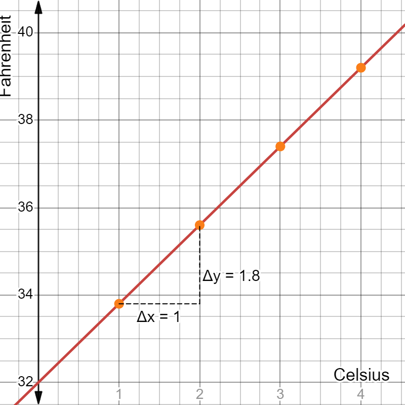
• The recipe says the oven should be at a certain temperature, given in Celsius, but you’re used to Fahrenheit:

\[Fahrenheit = 32 + 1.8 \times Celsius\]

Example: Cups to deciliters

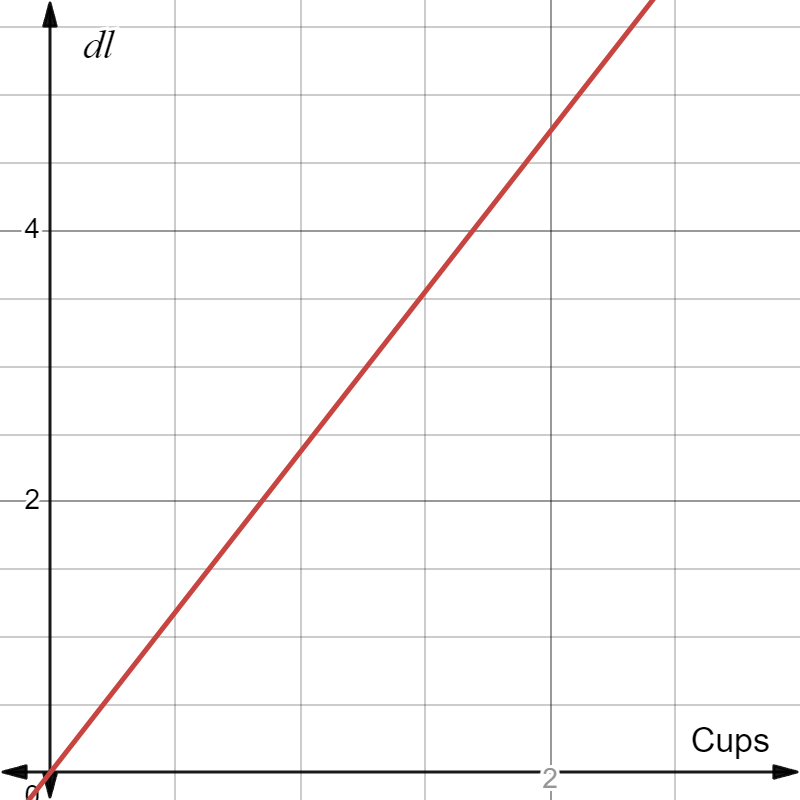
Example: Cups to deciliters

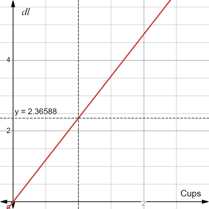
Example: Cups to deciliters

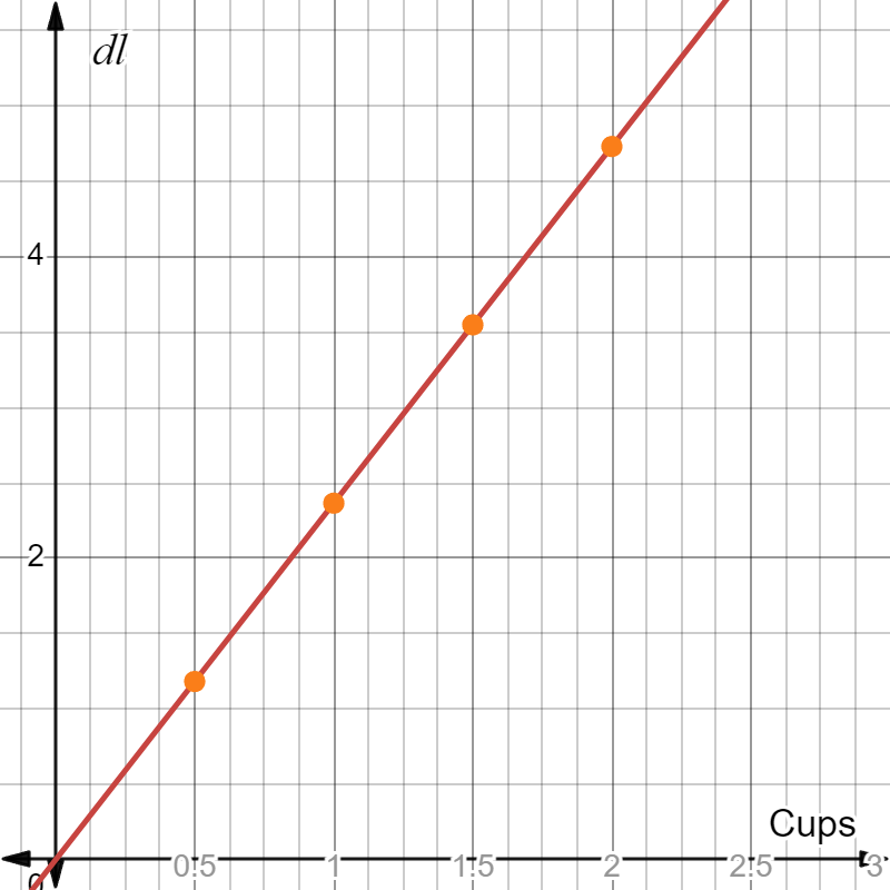
Linear relationship

• For every value on the \(x\)-axis (cups) we get a value on the \(y\)-axis
• Example: When \(cups = 1\), \(deciliter = 2.36588\); when \(cups = 2\), \(deciliter = 4.73176\)
• When \(cups = 0\), \(deciliter = 0\) (of course)
• However, \(x = 0\) doesn’t have to give \(y = 0\) for other relationships

Celsius to Fahrenheit

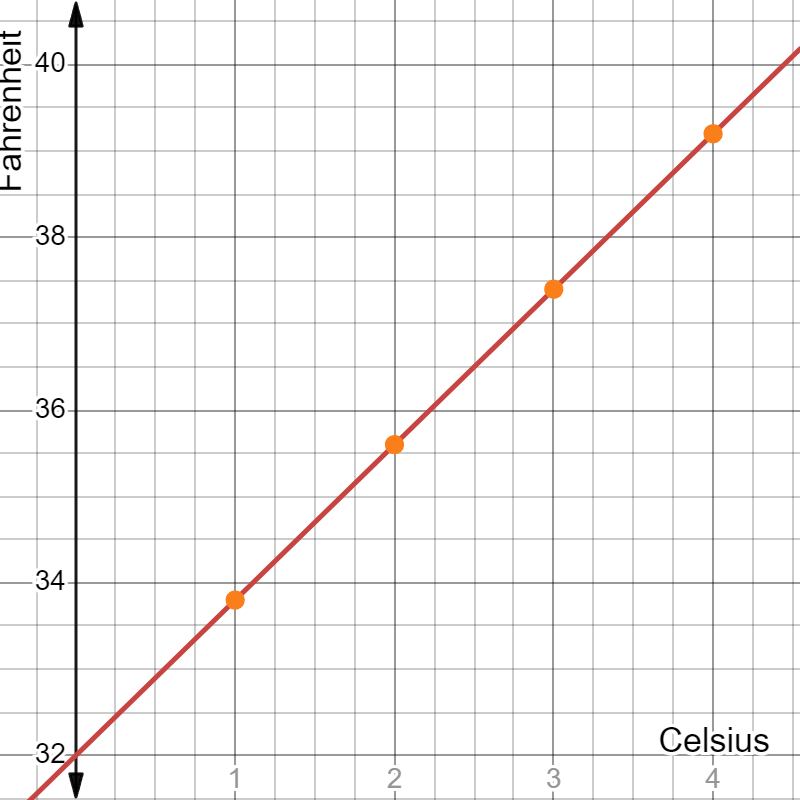
Celsius to Fahrenheit

Linear equation

• A linear relationship can be described with a linear equation:

\[y = kx + m\]

• The slope of the line is given by \(k\), while \(m\) is the constant
• Cups to deciliters: \(m = 0\) and \(k= 2.36588\)
• Celsius to Fahrenheit, \(m=32\) and \(k= 1.8\)

Linear equation

• In statistics a modified version is used

\[y = a + bx\]

• The slope, also called the slope coefficient, is given by \(b\), while \(a\) is the constant
• We call \(y\) the dependent variable, while \(x\) is called the independent variable
• If \(b\) is greater than zero, the relationship is positive
• If \(b\) is less than zero, the relationship is negative
• If \(b\) equals zero, there is no relationship

Positive, negative, or no relationship

// One-time (non-reactive) global listener: on mobile, rotating the
// screen fires "orientationchange" while iOS Safari is still mid-way
// through animating the address bar/viewport, so reveal.js's own
// resize handler picks up transitional (wrong) dimensions and mis-
// scales the slide -- which is what made every interactive figure
// disappear until a full reload. Re-running reveal.js's own layout
// pass a moment after rotation, once the viewport has settled, fixes
// this without touching any figure's own code.
orientationRelayout = {
  window.addEventListener("orientationchange", () => {
    setTimeout(() => {
      if (typeof Reveal !== "undefined" && Reveal.layout) Reveal.layout();
    }, 400);
  });
  return null;
}

mutable relType = null

html`<div class="rel-buttons-wrap">
  <div class="rel-buttons-title">Relationship</div>
  <div class="sd-buttons">
    ${Inputs.button("Positive", { value: null, reduce: () => { mutable relType = "pos"; return null; } })}
    ${Inputs.button("Negative", { value: null, reduce: () => { mutable relType = "neg"; return null; } })}
    ${Inputs.button("None", { value: null, reduce: () => { mutable relType = "none"; return null; } })}
  </div>
</div>`

html`<div class="rel-equation">${relType ? relEquation(relType) : ""}</div>`

relWidth = 640
relHeight = 500
relMarginLeft = 40
relMarginRight = 55
relMarginTop = 45
relMarginBottom = 30
relXDomain = [-0.4, 4.4]
relYDomain = [-1.3, 4.8]
relGridStep = 0.5

relXScale = d3.scaleLinear().domain(relXDomain).range([relMarginLeft, relWidth - relMarginRight])
relYScale = d3.scaleLinear().domain(relYDomain).range([relHeight - relMarginBottom, relMarginTop])

relXTicks = d3.range(Math.ceil(relXDomain[0] / relGridStep) * relGridStep, relXDomain[1] + 1e-9, relGridStep)
relYTicks = d3.range(Math.ceil(relYDomain[0] / relGridStep) * relGridStep, relYDomain[1] + 1e-9, relGridStep)

function relLineFn(type, x) {
  if (type === "pos") return 2 + 0.5 * x;
  if (type === "neg") return 2 - 0.5 * x;
  return 2;
}
function relColor(type) {
  return type === "pos" ? "#2563eb" : type === "neg" ? "#dc2626" : "#6b7280";
}
function relEquation(type) {
  if (type === "pos") return "Y = 2 + 0.5X";
  if (type === "neg") return "Y = 2 − 0.5X";
  return "Y = 2";
}

// Number formatter for the hover tooltip (e.g. "2.5"), trimming
// trailing zeros so whole numbers show as "1" not "1.00".
function svFmt(v) {
  const r = Math.round(v * 100) / 100;
  const s = r.toFixed(2).replace(/0+$/, "").replace(/\.$/, "");
  return s;
}

// Built fresh from scratch whenever relType changes (cheap -- no
// animation to preserve across redraws, unlike the CLT/pizza figures
// elsewhere in this deck), so hover/tap handlers below are always
// closures over the *current* relType and line.
relSvg = {
  const svg = d3.create("svg")
    .attr("viewBox", `0 0 ${relWidth} ${relHeight}`)
    .attr("width", relWidth)
    .attr("height", relHeight)
    .attr("class", "rel-svg")
    .style("touch-action", "none");

  const xAxisY = relYScale(0);
  const yAxisX = relXScale(0);

  const gridG = svg.append("g");
  for (const gx of relXTicks) {
    gridG.append("line")
      .attr("x1", relXScale(gx)).attr("x2", relXScale(gx))
      .attr("y1", relMarginTop).attr("y2", relHeight - relMarginBottom)
      .attr("stroke", "#e5e5e5").attr("stroke-width", 1);
  }
  for (const gy of relYTicks) {
    gridG.append("line")
      .attr("x1", relMarginLeft).attr("x2", relWidth - relMarginRight)
      .attr("y1", relYScale(gy)).attr("y2", relYScale(gy))
      .attr("stroke", "#e5e5e5").attr("stroke-width", 1);
  }

  svg.append("line")
    .attr("x1", relXScale(relXDomain[0])).attr("x2", relXScale(relXDomain[1]))
    .attr("y1", xAxisY).attr("y2", xAxisY)
    .attr("stroke", "#333").attr("stroke-width", 2);
  svg.append("line")
    .attr("x1", yAxisX).attr("x2", yAxisX)
    .attr("y1", relYScale(relYDomain[0])).attr("y2", relYScale(relYDomain[1]))
    .attr("stroke", "#333").attr("stroke-width", 2);

  const xTipX = relXScale(relXDomain[1]);
  svg.append("path")
    .attr("d", `M ${xTipX} ${xAxisY} L ${xTipX - 9} ${xAxisY - 5} L ${xTipX - 9} ${xAxisY + 5} Z`)
    .attr("fill", "#333");
  const yTipY = relYScale(relYDomain[1]);
  svg.append("path")
    .attr("d", `M ${yAxisX} ${yTipY} L ${yAxisX - 5} ${yTipY + 9} L ${yAxisX + 5} ${yTipY + 9} Z`)
    .attr("fill", "#333");

  svg.append("text")
    .attr("x", xTipX).attr("y", xAxisY + 22)
    .attr("text-anchor", "end").attr("font-size", 18).attr("font-weight", "bold")
    .attr("fill", "#333").text("X");
  svg.append("text")
    .attr("x", yAxisX - 10).attr("y", yTipY + 4)
    .attr("text-anchor", "end").attr("font-size", 18).attr("font-weight", "bold")
    .attr("fill", "#333").text("Y");

  // Numeric tick marks/labels along both axes. The x=0 label is
  // skipped here since the y-axis tick loop already draws a single
  // "0" right at the origin -- drawing it twice would just overlap.
  const tickG = svg.append("g");
  for (const gx of relXTicks) {
    if (gx === 0) continue;
    const px = relXScale(gx);
    tickG.append("line")
      .attr("x1", px).attr("x2", px)
      .attr("y1", xAxisY).attr("y2", xAxisY + 5)
      .attr("stroke", "#333").attr("stroke-width", 1);
    tickG.append("text")
      .attr("x", px).attr("y", xAxisY + 19)
      .attr("text-anchor", "middle").attr("font-size", 13)
      .attr("fill", "#555").text(svFmt(gx));
  }
  for (const gy of relYTicks) {
    const py = relYScale(gy);
    tickG.append("line")
      .attr("x1", yAxisX - 5).attr("x2", yAxisX)
      .attr("y1", py).attr("y2", py)
      .attr("stroke", "#333").attr("stroke-width", 1);
    // The origin's "0" sits diagonally down-left of the axis crossing
    // instead of directly left, so it doesn't crowd either axis line.
    if (gy === 0) {
      tickG.append("text")
        .attr("x", yAxisX - 10).attr("y", py + 16)
        .attr("text-anchor", "end").attr("font-size", 13)
        .attr("fill", "#555").text(svFmt(gy));
    } else {
      tickG.append("text")
        .attr("x", yAxisX - 9).attr("y", py + 4)
        .attr("text-anchor", "end").attr("font-size", 13)
        .attr("fill", "#555").text(svFmt(gy));
    }
  }

  if (relType) {
    const x0 = relXDomain[0], x1 = relXDomain[1];
    const y0 = relLineFn(relType, x0), y1 = relLineFn(relType, x1);
    svg.append("line")
      .attr("x1", relXScale(x0)).attr("y1", relYScale(y0))
      .attr("x2", relXScale(x1)).attr("y2", relYScale(y1))
      .attr("stroke", relColor(relType)).attr("stroke-width", 3);

    const hoverG = svg.append("g").attr("display", "none");
    // Dashed projection lines out to each axis, drawn first so the
    // dot/glow/text sit visually on top of them.
    const hoverGuideY = hoverG.append("line")
      .attr("stroke", relColor(relType)).attr("stroke-opacity", 0.55)
      .attr("stroke-width", 1).attr("stroke-dasharray", "4,3");
    const hoverGuideX = hoverG.append("line")
      .attr("stroke", relColor(relType)).attr("stroke-opacity", 0.55)
      .attr("stroke-width", 1).attr("stroke-dasharray", "4,3");
    hoverG.append("circle").attr("class", "rel-hover-glow").attr("r", 9)
      .attr("fill", relColor(relType)).attr("fill-opacity", 0.25);
    hoverG.append("circle").attr("class", "rel-hover-dot").attr("r", 4)
      .attr("fill", relColor(relType));
    const hoverText = hoverG.append("text")
      .attr("text-anchor", "middle")
      .attr("font-size", 14)
      .attr("fill", relColor(relType));

    function showHover(x, y) {
      const px = relXScale(x), py = relYScale(y);
      hoverG.attr("display", null);
      // Out to the y-axis (horizontal) and down to the x-axis (vertical).
      hoverGuideY.attr("x1", px).attr("y1", py).attr("x2", yAxisX).attr("y2", py);
      hoverGuideX.attr("x1", px).attr("y1", py).attr("x2", px).attr("y2", xAxisY);
      hoverG.select(".rel-hover-glow").attr("cx", px).attr("cy", py);
      hoverG.select(".rel-hover-dot").attr("cx", px).attr("cy", py);
      hoverText.attr("x", px).attr("y", py - 14).text(`X = ${svFmt(x)}, Y = ${svFmt(y)}`);
    }
    function hideHover() {
      hoverG.attr("display", "none");
    }

    // Snap-candidates are the line's own points at each relGridStep
    // x-step (the same spacing as the background grid). Pixel radius is
    // derived from the actual on-screen spacing between them, kept
    // just under half a step, so neighbouring points never fight over
    // the same pointer position.
    const pixelStep = Math.abs(relXScale(relGridStep) - relXScale(0));
    const mouseRadius = pixelStep * 0.45;
    const touchRadius = pixelStep * 0.48;

    function nearestCandidate(mx, my) {
      let best = null, bestDist = Infinity;
      for (const gx of relXTicks) {
        const gy = relLineFn(relType, gx);
        const px = relXScale(gx), py = relYScale(gy);
        const d = Math.hypot(px - mx, py - my);
        if (d < bestDist) { bestDist = d; best = { x: gx, y: gy, dist: d }; }
      }
      return best;
    }

    const overlay = svg.append("rect")
      .attr("x", relMarginLeft).attr("y", relMarginTop)
      .attr("width", relWidth - relMarginLeft - relMarginRight)
      .attr("height", relHeight - relMarginTop - relMarginBottom)
      .attr("fill", "transparent")
      .style("cursor", "pointer");

    // Mouse/pen: continuous hover as the pointer moves.
    overlay.on("pointermove", (event) => {
      if (event.pointerType === "touch") return;
      const [mx, my] = d3.pointer(event);
      const cand = nearestCandidate(mx, my);
      if (cand && cand.dist <= mouseRadius) showHover(cand.x, cand.y);
      else hideHover();
    });
    overlay.on("pointerleave", () => hideHover());

    // Touch (and mouse, harmlessly): tap to show, tap elsewhere to hide.
    overlay.on("click", (event) => {
      const [mx, my] = d3.pointer(event);
      const cand = nearestCandidate(mx, my);
      if (cand && cand.dist <= touchRadius) showHover(cand.x, cand.y);
      else hideHover();
    });
  }

  return svg.node();
}

html`<div class="ojs-plot-wrap">${relSvg}</div>`

Linear equation

• So far we’ve seen examples of an exact linear relationship
• The dots represent our data: all dots lie on the line
• Relationships are rarely exact, though; usually they are inexact
• This can be because we can’t always make exact measurements
• More likely, though, is that we’re studying complex relationships

Income and indoor temperature

• Back to our scenario: we want to understand what determines which indoor temperature households choose to have
• Those with higher income are more likely to be able to afford higher electricity costs
• Reasonable to assume a positive relationship between income and indoor temperature
• But we shouldn’t assume the relationship is exact, since households’ indoor temperature is also affected by other factors

Example: temperature data

• Suppose we have a random sample of 15 households

Household ID	Indoor temperature	Monthly income (in thousands of SEK)
1	18.3	13.4
2	19.5	13.6
3	20.5	26.9
4	20.8	33.5
5	18.5	14.4
6	20.4	44.0
7	17.2	20.3
8	15.9	16.6
9	22.3	28.8
10	16.6	35.0
11	21.6	28.9
12	25.4	42.3
13	19.7	27.8
14	23.5	24.7
15	18.0	29.2

Is there a linear relationship?

• It looks like those with higher income also have higher indoor temperature
• However, it’s probably not an exact linear relationship
• We need a modified equation to account for the relationship not being exact:

\[Y_i = a + b X_i + e_i\]

• The parameters \(a\) and \(b\) represent the constant (intercept) and the slope coefficient, just as in the previous equation
• The error term \(e_i\) compensates for the fact that the observations deviate from the straight line

Explore the data: temperature and income

• Graph
• Data

mutable selectedHH = null

// One-time (non-reactive, no dependencies -- runs exactly once) global
// listener: clicking anywhere that isn't a data point or a Data-tab
// table row closes the currently open info box and returns to plain
// hover mode.
hhClickAwayListener = {
  document.addEventListener("click", (event) => {
    if (event.target.closest(".hh-dot, .hh-hit, .hh-row")) return;
    mutable selectedHH = null;
  });
  return null;
}

hhData = [
  {id: 1, temp: 18.3, income: 13.4},
  {id: 2, temp: 19.5, income: 13.6},
  {id: 3, temp: 20.5, income: 26.9},
  {id: 4, temp: 20.8, income: 33.5},
  {id: 5, temp: 18.5, income: 14.4},
  {id: 6, temp: 20.4, income: 44.0},
  {id: 7, temp: 17.2, income: 20.3},
  {id: 8, temp: 15.9, income: 16.6},
  {id: 9, temp: 22.3, income: 28.8},
  {id: 10, temp: 16.6, income: 35.0},
  {id: 11, temp: 21.6, income: 28.9},
  {id: 12, temp: 25.4, income: 42.3},
  {id: 13, temp: 19.7, income: 27.8},
  {id: 14, temp: 23.5, income: 24.7},
  {id: 15, temp: 18.0, income: 29.2}
]

// Formatter for this figure specifically: always one decimal (e.g.
// "44.0", not "44"), so numbers line up visually with the printed
// table on the previous slide instead of dropping trailing zeros like
// svFmt does on the Positive/Negative figure.
function hhFmt(v) {
  return v.toFixed(1);
}

hhWidth = 760
hhHeight = 460
hhMarginLeft = 46
hhMarginRight = 20
hhMarginTop = 22
hhMarginBottom = 40
hhXDomain = [-2.5, 51]
hhYDomain = [14.5, 25.8]
hhXStep = 2
hhYStep = 1
hhXLabelStep = 10
hhYLabelStep = 5

hhXScale = d3.scaleLinear().domain(hhXDomain).range([hhMarginLeft, hhWidth - hhMarginRight])
hhYScale = d3.scaleLinear().domain(hhYDomain).range([hhHeight - hhMarginBottom, hhMarginTop])

hhXTicks = d3.range(Math.ceil(hhXDomain[0] / hhXStep) * hhXStep, hhXDomain[1] + 1e-9, hhXStep)
hhYTicks = d3.range(Math.ceil(hhYDomain[0] / hhYStep) * hhYStep, hhYDomain[1] + 1e-9, hhYStep)

mutable showRegLine = false

html`<div class="sd-buttons-wrap">
  <div class="sd-buttons">
    ${Inputs.button(showRegLine ? "Hide regression line" : "Show regression line", {
      value: null,
      reduce: () => { mutable showRegLine = !showRegLine; return null; }
    })}
  </div>
</div>`

// Rebuilt whenever selectedHH or showRegLine changes (click on a dot,
// a jump from the Data tab's table, or the regression-line button) --
// cheap with only 15 points, so no need for the imperative-DOM-patching
// approach used on continuous-hover figures elsewhere in this deck.
hhSvg = {
  const svg = d3.create("svg")
    .attr("viewBox", `0 0 ${hhWidth} ${hhHeight}`)
    .attr("width", hhWidth)
    .attr("height", hhHeight)
    .attr("class", "hh-svg")
    .style("touch-action", "none");

  const xAxisY = hhYScale(hhYDomain[0]);
  const yAxisX = hhXScale(hhXDomain[0]);

  const gridG = svg.append("g");
  for (const gx of hhXTicks) {
    gridG.append("line")
      .attr("x1", hhXScale(gx)).attr("x2", hhXScale(gx))
      .attr("y1", hhMarginTop).attr("y2", xAxisY)
      .attr("stroke", "#e5e5e5").attr("stroke-width", 1);
  }
  for (const gy of hhYTicks) {
    gridG.append("line")
      .attr("x1", yAxisX).attr("x2", hhWidth - hhMarginRight)
      .attr("y1", hhYScale(gy)).attr("y2", hhYScale(gy))
      .attr("stroke", "#e5e5e5").attr("stroke-width", 1);
  }

  svg.append("line")
    .attr("x1", yAxisX).attr("x2", hhWidth - hhMarginRight)
    .attr("y1", xAxisY).attr("y2", xAxisY)
    .attr("stroke", "#333").attr("stroke-width", 2);
  svg.append("line")
    .attr("x1", yAxisX).attr("x2", yAxisX)
    .attr("y1", hhMarginTop).attr("y2", xAxisY)
    .attr("stroke", "#333").attr("stroke-width", 2);

  // Tick marks every hhXStep/hhYStep, but numeric labels only every
  // hhXLabelStep/hhYLabelStep -- so the grid is finer than what's
  // actually labelled.
  const tickG = svg.append("g");
  for (const gx of hhXTicks) {
    tickG.append("line")
      .attr("x1", hhXScale(gx)).attr("x2", hhXScale(gx))
      .attr("y1", xAxisY).attr("y2", xAxisY + 5)
      .attr("stroke", "#333").attr("stroke-width", 1);
    if (Math.round(gx) % hhXLabelStep === 0) {
      tickG.append("text")
        .attr("x", hhXScale(gx)).attr("y", xAxisY + 19)
        .attr("text-anchor", "middle").attr("font-size", 14)
        .attr("fill", "#555").text(String(gx));
    }
  }
  for (const gy of hhYTicks) {
    tickG.append("line")
      .attr("x1", yAxisX - 5).attr("x2", yAxisX)
      .attr("y1", hhYScale(gy)).attr("y2", hhYScale(gy))
      .attr("stroke", "#333").attr("stroke-width", 1);
    if (Math.round(gy) % hhYLabelStep === 0) {
      tickG.append("text")
        .attr("x", yAxisX - 10).attr("y", hhYScale(gy) + 5)
        .attr("text-anchor", "end").attr("font-size", 14)
        .attr("fill", "#555").text(String(gy));
    }
  }

  // "Income" sits near the right end of the x-axis (anchor="end" so
  // it ends just inside the right edge instead of overflowing past
  // it). "Temperature" sits near the top of the y-axis, close to the
  // "25" tick -- rotate(-90) around a point near the top plus
  // anchor="end" makes the text extend *downward* from that point
  // (not upward off the top edge of the figure).
  svg.append("text")
    .attr("x", hhWidth - hhMarginRight - 4)
    .attr("y", xAxisY - 6)
    .attr("text-anchor", "end").attr("font-size", 16).attr("font-weight", "bold")
    .attr("fill", "#333").text("Income");

  const yLabelAnchorY = hhMarginTop + 10;
  svg.append("text")
    .attr("x", yAxisX + 18).attr("y", yLabelAnchorY)
    .attr("transform", `rotate(-90, ${yAxisX + 18}, ${yLabelAnchorY})`)
    .attr("text-anchor", "end").attr("font-size", 16).attr("font-weight", "bold")
    .attr("fill", "#333").text("Temperature");

  // Regression line drawn before the dots (not after), so the data
  // points always sit visually on top of it.
  if (showRegLine) {
    const rx0 = hhXDomain[0], rx1 = hhXDomain[1];
    const ry0 = 16.43 + 0.13 * rx0, ry1 = 16.43 + 0.13 * rx1;
    svg.append("line")
      .attr("x1", hhXScale(rx0)).attr("y1", hhYScale(ry0))
      .attr("x2", hhXScale(rx1)).attr("y2", hhYScale(ry1))
      .attr("stroke", "#16a34a").attr("stroke-width", 2.5);
  }

  const dotsG = svg.append("g");
  const infoG = svg.append("g");

  function renderInfoBox(id) {
    infoG.selectAll("*").remove();
    const d = hhData.find(h => h.id === id);
    if (!d) return;
    const px = hhXScale(d.income), py = hhYScale(d.temp);
    const boxW = 128, boxH = 58;
    let bx = px + 10, by = py - boxH - 8;
    if (bx + boxW > hhWidth - 2) bx = px - boxW - 10;
    if (by < 2) by = py + 10;
    infoG.append("rect")
      .attr("x", bx).attr("y", by).attr("width", boxW).attr("height", boxH)
      .attr("rx", 6).attr("fill", "white").attr("fill-opacity", 0.95)
      .attr("stroke", "#999").attr("stroke-width", 1);
    const lines = [
      `Household: ${d.id}`,
      `Temperature: ${hhFmt(d.temp)}`,
      `Income: ${hhFmt(d.income)}`
    ];
    lines.forEach((line, i) => {
      infoG.append("text")
        .attr("x", bx + 8).attr("y", by + 18 + i * 16)
        .attr("font-size", 12).attr("fill", "#333").text(line);
    });
  }

  const circleSel = dotsG.selectAll("circle")
    .data(hhData)
    .join("circle")
    .attr("class", "hh-dot")
    .attr("cx", d => hhXScale(d.income))
    .attr("cy", d => hhYScale(d.temp))
    .attr("fill-opacity", 0.85);

  function setDotStyle(id) {
    circleSel
      .attr("r", d => d.id === id ? 6 : 4)
      .attr("fill", d => d.id === id ? "#dc2626" : "#2563eb");
  }

  // Initial state reflects the *persistent* selection only (a click, or
  // a jump from the Data tab's table) -- this is the mutable-driven,
  // reactive part, rebuilt whenever selectedHH changes.
  setDotStyle(selectedHH);
  renderInfoBox(selectedHH);

  // Invisible, much larger hit-circles sit on top of the tiny visible
  // dots and carry all the pointer/click handlers -- a 4-6px visible
  // dot is far below the ~44px touch target Apple/Google recommend, so
  // tapping it accurately on a phone was close to impossible.
  const hitSel = dotsG.selectAll("circle.hh-hit")
    .data(hhData)
    .join("circle")
    .attr("class", "hh-hit")
    .attr("cx", d => hhXScale(d.income))
    .attr("cy", d => hhYScale(d.temp))
    .attr("r", 15)
    .attr("fill", "transparent")
    .style("cursor", "pointer");

  // Hover (mouse only -- touch has no hover state, so it's handled by
  // "click" below) is deliberately kept OUT of the mutable/reactive
  // graph: setting `mutable selectedHH` on pointerenter would rebuild
  // this whole SVG mid-hover, replacing the very circle the pointer is
  // sitting on, which silently suppressed the browser's own
  // pointerleave event and left the box stuck open. Direct DOM
  // manipulation instead keeps the actual hovered element alive for
  // its own pointerleave to fire normally, so moving the pointer away
  // -- even to empty space, not just onto another dot -- always closes
  // it. Once a selection is *locked in* (via a click, or a jump from
  // the Data tab's table), hover is ignored entirely instead of
  // transiently overriding it and then snapping back on pointerleave
  // -- that snap-back read as flickery/distracting. A locked box only
  // changes via a new click, or gets cleared by the page's click-away
  // listener (which also fires when switching back to the Data tab,
  // since that click isn't on a dot or a row either).
  hitSel
    .on("pointerenter", (event, d) => {
      if (event.pointerType === "touch") return;
      if (selectedHH !== null) return;
      setDotStyle(d.id);
      renderInfoBox(d.id);
    })
    .on("pointerleave", (event) => {
      if (event.pointerType === "touch") return;
      if (selectedHH !== null) return;
      setDotStyle(null);
      renderInfoBox(null);
    })
    .on("click", (event, d) => {
      mutable selectedHH = d.id;
    });

  return svg.node();
}

html`<div class="ojs-plot-wrap">${hhSvg}</div>`

html`<div class="hh-reg-note">${showRegLine ? "Predicted temperature: Ŷ = 16.43 + 0.13 × X" : ""}</div>`

// Built with D3 (not a plain markdown table) so each row can get a real
// click listener -- clicking a row jumps to the Graph tab (by clicking
// its tab link, letting the tabby library handle the actual switch) and
// selects that household's point, popping its info box open.
hhTable = {
  const wrap = d3.create("div").attr("class", "hh-table-wrap");
  const table = wrap.append("table").attr("class", "hh-data-table");
  table.append("thead").append("tr")
    .selectAll("th")
    .data(["Household ID", "Indoor temperature", "Monthly income (in thousands of SEK)"])
    .join("th")
    .text(d => d);
  const tbody = table.append("tbody");
  hhData.forEach(d => {
    const tr = tbody.append("tr").attr("class", "hh-row");
    tr.append("td").text(d.id);
    tr.append("td").text(hhFmt(d.temp));
    tr.append("td").text(hhFmt(d.income));
    tr.on("click", () => {
      // The tab link's own (synthetic) click also bubbles to the
      // document-level "click away" listener above, which would clear
      // selectedHH right back out -- so it must run *before* we set
      // the real value, not after.
      const tabsetEl = document.querySelector(".hh-graph-tabset");
      const firstLink = tabsetEl && tabsetEl.querySelector(".panel-tabset-tabby li:first-child a");
      if (firstLink) firstLink.click();
      mutable selectedHH = d.id;
    });
  });
  return wrap.node();
}

The regression line

• The regression line is meant to fit our data and is given by the equation:

\[\hat{Y_i} = 16.43+0.13 \times X_i\]

• The “hat” on \(Y_i\) indicates that this is the model’s estimate (or prediction) of \(Y_i\)
• The slope coefficient (\(b\)) measures the slope of the regression line, and in this case equals 0.13
• Interpretation of the slope coefficient: a one-unit increase in \(X\) is expected to increase \(Y\) by 0.13 units
• In our example: an increase of 1000 SEK (why?) is expected to increase indoor temperature by 0.13 degrees Celsius

Predicting the indoor temperature

• The constant (intercept) equals 16.43
• Interpretation of the constant: when income equals 0, the room temperature is expected to equal 16.43
• There isn’t always a sensible interpretation of the constant (what does 0 income mean?)
• Example: expected indoor temperature for a household with a monthly income of 30,000 SEK: 16.43 \(+\) 0.13 \(\times\) 30 \(=\) 20.33
• But wait: how do we choose the regression line?
• Isn’t there another line that fits the data better?

Other possible lines

• What about these lines?

cmpWidth = 760
cmpHeight = 460
cmpMarginLeft = 46
cmpMarginRight = 20
cmpMarginTop = 22
cmpMarginBottom = 40
cmpXDomain = [-2.5, 51]
cmpYDomain = [14.5, 25.8]
cmpXStep = 2
cmpYStep = 1
cmpXLabelStep = 10
cmpYLabelStep = 5

cmpXScale = d3.scaleLinear().domain(cmpXDomain).range([cmpMarginLeft, cmpWidth - cmpMarginRight])
cmpYScale = d3.scaleLinear().domain(cmpYDomain).range([cmpHeight - cmpMarginBottom, cmpMarginTop])

cmpXTicks = d3.range(Math.ceil(cmpXDomain[0] / cmpXStep) * cmpXStep, cmpXDomain[1] + 1e-9, cmpXStep)
cmpYTicks = d3.range(Math.ceil(cmpYDomain[0] / cmpYStep) * cmpYStep, cmpYDomain[1] + 1e-9, cmpYStep)

// Three plausible-but-wrong alternative fits (none is the actual
// least-squares line), listed in hover-priority order: where two
// lines' hit areas overlap, the first one in this array wins.
cmpLines = [
  { a: 15.2, b: 0.16, color: "#2563eb", dash: "7,5" },
  { a: 18.1, b: 0.09, color: "#b45309", dash: "1.5,4" },
  { a: 14.8, b: 0.19, color: "#15803d", dash: null }
]

function cmpFmt(v, decimals = 2) {
  return v.toFixed(decimals);
}

function distToSegment(px, py, x1, y1, x2, y2) {
  const dx = x2 - x1, dy = y2 - y1;
  const lenSq = dx * dx + dy * dy;
  let t = lenSq === 0 ? 0 : ((px - x1) * dx + (py - y1) * dy) / lenSq;
  t = Math.max(0, Math.min(1, t));
  const cx = x1 + t * dx, cy = y1 + t * dy;
  return Math.hypot(px - cx, py - cy);
}

// Reuses hhData (defined once, on the "Explore the data" slide) --
// points here are plain and non-interactive (no per-observation info
// boxes, removed to keep this figure from getting too busy alongside
// the three line tooltips).
cmpSvg = {
  const svg = d3.create("svg")
    .attr("viewBox", `0 0 ${cmpWidth} ${cmpHeight}`)
    .attr("width", cmpWidth)
    .attr("height", cmpHeight)
    .attr("class", "cmp-svg")
    .style("touch-action", "none");

  const xAxisY = cmpYScale(cmpYDomain[0]);
  const yAxisX = cmpXScale(cmpXDomain[0]);

  const gridG = svg.append("g");
  for (const gx of cmpXTicks) {
    gridG.append("line")
      .attr("x1", cmpXScale(gx)).attr("x2", cmpXScale(gx))
      .attr("y1", cmpMarginTop).attr("y2", xAxisY)
      .attr("stroke", "#e5e5e5").attr("stroke-width", 1);
  }
  for (const gy of cmpYTicks) {
    gridG.append("line")
      .attr("x1", yAxisX).attr("x2", cmpWidth - cmpMarginRight)
      .attr("y1", cmpYScale(gy)).attr("y2", cmpYScale(gy))
      .attr("stroke", "#e5e5e5").attr("stroke-width", 1);
  }

  svg.append("line")
    .attr("x1", yAxisX).attr("x2", cmpWidth - cmpMarginRight)
    .attr("y1", xAxisY).attr("y2", xAxisY)
    .attr("stroke", "#333").attr("stroke-width", 2);
  svg.append("line")
    .attr("x1", yAxisX).attr("x2", yAxisX)
    .attr("y1", cmpMarginTop).attr("y2", xAxisY)
    .attr("stroke", "#333").attr("stroke-width", 2);

  const tickG = svg.append("g");
  for (const gx of cmpXTicks) {
    tickG.append("line")
      .attr("x1", cmpXScale(gx)).attr("x2", cmpXScale(gx))
      .attr("y1", xAxisY).attr("y2", xAxisY + 5)
      .attr("stroke", "#333").attr("stroke-width", 1);
    if (Math.round(gx) % cmpXLabelStep === 0) {
      tickG.append("text")
        .attr("x", cmpXScale(gx)).attr("y", xAxisY + 19)
        .attr("text-anchor", "middle").attr("font-size", 14)
        .attr("fill", "#555").text(String(gx));
    }
  }
  for (const gy of cmpYTicks) {
    tickG.append("line")
      .attr("x1", yAxisX - 5).attr("x2", yAxisX)
      .attr("y1", cmpYScale(gy)).attr("y2", cmpYScale(gy))
      .attr("stroke", "#333").attr("stroke-width", 1);
    if (Math.round(gy) % cmpYLabelStep === 0) {
      tickG.append("text")
        .attr("x", yAxisX - 10).attr("y", cmpYScale(gy) + 5)
        .attr("text-anchor", "end").attr("font-size", 14)
        .attr("fill", "#555").text(String(gy));
    }
  }

  svg.append("text")
    .attr("x", cmpWidth - cmpMarginRight - 4)
    .attr("y", xAxisY - 6)
    .attr("text-anchor", "end").attr("font-size", 16).attr("font-weight", "bold")
    .attr("fill", "#333").text("Income");

  const yLabelAnchorY = cmpMarginTop + 10;
  svg.append("text")
    .attr("x", yAxisX + 18).attr("y", yLabelAnchorY)
    .attr("transform", `rotate(-90, ${yAxisX + 18}, ${yLabelAnchorY})`)
    .attr("text-anchor", "end").attr("font-size", 16).attr("font-weight", "bold")
    .attr("fill", "#333").text("Temperature");

  const lineEls = cmpLines.map(ln => {
    const x0 = cmpXDomain[0], x1 = cmpXDomain[1];
    const y0 = ln.a + ln.b * x0, y1 = ln.a + ln.b * x1;
    const sel = svg.append("line")
      .attr("x1", cmpXScale(x0)).attr("y1", cmpYScale(y0))
      .attr("x2", cmpXScale(x1)).attr("y2", cmpYScale(y1))
      .attr("stroke", ln.color).attr("stroke-width", 2.5);
    if (ln.dash) sel.attr("stroke-dasharray", ln.dash);
    return { ...ln, x1p: cmpXScale(x0), y1p: cmpYScale(y0), x2p: cmpXScale(x1), y2p: cmpYScale(y1) };
  });

  const dotsG = svg.append("g");
  dotsG.selectAll("circle")
    .data(hhData)
    .join("circle")
    .attr("cx", d => cmpXScale(d.income))
    .attr("cy", d => cmpYScale(d.temp))
    .attr("r", 4)
    .attr("fill", "#6b7280")
    .attr("fill-opacity", 0.8);

  const tipG = svg.append("g").attr("display", "none");
  const tipRect = tipG.append("rect")
    .attr("rx", 6).attr("fill", "white").attr("fill-opacity", 0.95).attr("stroke-width", 1.5);
  const tipText = tipG.append("text").attr("font-size", 13);

  function showTip(mx, my, ln) {
    const label = `Ŷ = ${cmpFmt(ln.a)} + ${cmpFmt(ln.b)} × X`;
    tipText.text(label).attr("fill", ln.color);
    const boxW = label.length * 7.6 + 18;
    const boxH = 26;
    let bx = mx + 12, by = my - boxH - 8;
    if (bx + boxW > cmpWidth - 2) bx = mx - boxW - 12;
    if (by < 2) by = my + 12;
    tipRect.attr("x", bx).attr("y", by).attr("width", boxW).attr("height", boxH).attr("stroke", ln.color);
    tipText.attr("x", bx + 9).attr("y", by + 17);
    tipG.attr("display", null);
  }
  function hideTip() {
    tipG.attr("display", "none");
  }

  // Priority order = cmpLines order: where two lines' hit areas
  // overlap (near a crossing), the first match in the array wins.
  const hitRadius = 12;
  function findLine(mx, my) {
    for (const ln of lineEls) {
      if (distToSegment(mx, my, ln.x1p, ln.y1p, ln.x2p, ln.y2p) <= hitRadius) return ln;
    }
    return null;
  }

  const overlay = svg.append("rect")
    .attr("x", cmpMarginLeft).attr("y", cmpMarginTop)
    .attr("width", cmpWidth - cmpMarginLeft - cmpMarginRight)
    .attr("height", cmpHeight - cmpMarginTop - cmpMarginBottom)
    .attr("fill", "transparent");

  overlay.on("pointermove", (event) => {
    if (event.pointerType === "touch") return;
    const [mx, my] = d3.pointer(event);
    const ln = findLine(mx, my);
    if (ln) showTip(mx, my, ln); else hideTip();
  });
  overlay.on("pointerleave", () => hideTip());
  overlay.on("click", (event) => {
    const [mx, my] = d3.pointer(event);
    const ln = findLine(mx, my);
    if (ln) showTip(mx, my, ln); else hideTip();
  });

  return svg.node();
}

html`<div class="ojs-plot-wrap">${cmpSvg}</div>`

The method of least squares

• The method of least squares gives us the line that minimizes the sum of squared deviations
• Every observation will deviate from the model’s prediction (the regression line)
• The method of least squares finds the line that makes the sum of the squared deviations as small as possible
• These deviations are called residuals and equal the actual value minus the predicted value:

\[\hat{e}_i = Y_i - \hat{Y_i}\]

Deviations from the regression line

• Graph
• Data

mutable residA = 16.43

mutable residB = 0.13

mutable residSelected = null

// A raw <input type="range"> + our own <span> readout, built by hand
// instead of via Inputs.range: this slide needs *two* independent
// copies of each slider (one in the Graph tab, one in the Data tab, see
// residSliderSync below) kept in sync with each other, which is far
// simpler to reason about with plain DOM elements we fully control
// than by fighting Inputs' own internal markup for a second instance.
function makeSlider(labelText, min, max, step, initial) {
  const wrap = document.createElement("div");
  wrap.className = "resid-slider";
  const label = document.createElement("span");
  label.className = "resid-slider-label";
  label.textContent = labelText;
  const input = document.createElement("input");
  input.type = "range";
  input.min = min; input.max = max; input.step = step; input.value = initial;
  const out = document.createElement("span");
  out.className = "resid-slider-value";
  out.textContent = cmpFmt(initial);
  wrap.append(input, out, label);
  return { wrap, input, out };
}

// Each pair is built once (no dependency on residA/residB), so
// dragging never tears down and rebuilds the input mid-gesture.
residSliderPairGraf = {
  const a = makeSlider("Intercept (a)", 5, 30, 0.01, 16.43);
  a.input.addEventListener("input", () => { mutable residA = Number(a.input.value); });
  const b = makeSlider("Slope coefficient (b)", -0.2, 0.5, 0.01, 0.13);
  b.input.addEventListener("input", () => { mutable residB = Number(b.input.value); });
  return { a, b };
}

residSliderPairData = {
  const a = makeSlider("Intercept (a)", 5, 30, 0.01, 16.43);
  a.input.addEventListener("input", () => { mutable residA = Number(a.input.value); });
  const b = makeSlider("Slope coefficient (b)", -0.2, 0.5, 0.01, 0.13);
  b.input.addEventListener("input", () => { mutable residB = Number(b.input.value); });
  return { a, b };
}

// Keeps *both* slider pairs' displayed position/text in sync with
// residA/residB, regardless of which pair (or the OLS button) caused
// the change -- this is what makes "what you change in one tab's
// sliders carries over to the other tab" actually true, since tabby
// only hides the inactive tab's DOM rather than destroying it (so an
// untouched copy would otherwise sit stale at its original value).
// Setting .value directly (not recreating the element) is safe to do
// even on the slider currently being dragged.
residSliderSync = {
  for (const pair of [residSliderPairGraf, residSliderPairData]) {
    if (Number(pair.a.input.value) !== residA) pair.a.input.value = residA;
    pair.a.out.textContent = cmpFmt(residA);
    if (Number(pair.b.input.value) !== residB) pair.b.input.value = residB;
    pair.b.out.textContent = cmpFmt(residB);
  }
  return null;
}

html`<div class="resid-sliders-row">${residSliderPairGraf.a.wrap}${residSliderPairGraf.b.wrap}</div>`

html`<div class="sd-buttons-wrap"><div class="sd-buttons">${
  Inputs.button("The least-squares regression line", {
    value: null,
    reduce: () => {
      mutable residA = 16.43;
      mutable residB = 0.13;
      return null;
    }
  })
}</div></div>`

// Sum of squared deviations for the *current* slider values -- this is
// exactly what the least-squares line minimizes.
residSSE = hhData.reduce((acc, d) => {
  const pred = residA + residB * d.income;
  return acc + (d.temp - pred) ** 2;
}, 0)

// Reuses hhData/hhFmt/hhXScale/hhYScale/hhXTicks/hhYTicks/hhWidth/
// hhHeight/hhMargin*/hhXDomain/hhYDomain/hhXLabelStep/hhYLabelStep from
// the "Explore the data" slide -- same axes, grid, and ticks by
// construction, not just by copying numbers. Rebuilt whenever residA,
// residB, or residSelected changes: the first two are cheap, desired
// full redraws (that's the whole point -- the line should visibly move
// as the sliders move), same reasoning as the "Other possible lines"
// slide's static lines. Hover (mouse) still avoids the mutable/reactive
// path -- see the "Explore the data" slide's own hhSvg for why:
// replacing the hovered circle mid-hover breaks the browser's own
// pointerleave event.
residSvg = {
  const svg = d3.create("svg")
    .attr("viewBox", `0 0 ${hhWidth} ${hhHeight}`)
    .attr("width", hhWidth)
    .attr("height", hhHeight)
    .attr("class", "resid-svg")
    .style("touch-action", "none");

  const xAxisY = hhYScale(hhYDomain[0]);
  const yAxisX = hhXScale(hhXDomain[0]);

  const gridG = svg.append("g");
  for (const gx of hhXTicks) {
    gridG.append("line")
      .attr("x1", hhXScale(gx)).attr("x2", hhXScale(gx))
      .attr("y1", hhMarginTop).attr("y2", xAxisY)
      .attr("stroke", "#e5e5e5").attr("stroke-width", 1);
  }
  for (const gy of hhYTicks) {
    gridG.append("line")
      .attr("x1", yAxisX).attr("x2", hhWidth - hhMarginRight)
      .attr("y1", hhYScale(gy)).attr("y2", hhYScale(gy))
      .attr("stroke", "#e5e5e5").attr("stroke-width", 1);
  }

  svg.append("line")
    .attr("x1", yAxisX).attr("x2", hhWidth - hhMarginRight)
    .attr("y1", xAxisY).attr("y2", xAxisY)
    .attr("stroke", "#333").attr("stroke-width", 2);
  svg.append("line")
    .attr("x1", yAxisX).attr("x2", yAxisX)
    .attr("y1", hhMarginTop).attr("y2", xAxisY)
    .attr("stroke", "#333").attr("stroke-width", 2);

  const tickG = svg.append("g");
  for (const gx of hhXTicks) {
    tickG.append("line")
      .attr("x1", hhXScale(gx)).attr("x2", hhXScale(gx))
      .attr("y1", xAxisY).attr("y2", xAxisY + 5)
      .attr("stroke", "#333").attr("stroke-width", 1);
    if (Math.round(gx) % hhXLabelStep === 0) {
      tickG.append("text")
        .attr("x", hhXScale(gx)).attr("y", xAxisY + 19)
        .attr("text-anchor", "middle").attr("font-size", 14)
        .attr("fill", "#555").text(String(gx));
    }
  }
  for (const gy of hhYTicks) {
    tickG.append("line")
      .attr("x1", yAxisX - 5).attr("x2", yAxisX)
      .attr("y1", hhYScale(gy)).attr("y2", hhYScale(gy))
      .attr("stroke", "#333").attr("stroke-width", 1);
    if (Math.round(gy) % hhYLabelStep === 0) {
      tickG.append("text")
        .attr("x", yAxisX - 10).attr("y", hhYScale(gy) + 5)
        .attr("text-anchor", "end").attr("font-size", 14)
        .attr("fill", "#555").text(String(gy));
    }
  }

  svg.append("text")
    .attr("x", hhWidth - hhMarginRight - 4)
    .attr("y", xAxisY - 6)
    .attr("text-anchor", "end").attr("font-size", 16).attr("font-weight", "bold")
    .attr("fill", "#333").text("Income");

  const yLabelAnchorY = hhMarginTop + 10;
  svg.append("text")
    .attr("x", yAxisX + 18).attr("y", yLabelAnchorY)
    .attr("transform", `rotate(-90, ${yAxisX + 18}, ${yLabelAnchorY})`)
    .attr("text-anchor", "end").attr("font-size", 16).attr("font-weight", "bold")
    .attr("fill", "#333").text("Temperature");

  function predY(x) { return residA + residB * x; }

  const rx0 = hhXDomain[0], rx1 = hhXDomain[1];
  svg.append("line")
    .attr("x1", hhXScale(rx0)).attr("y1", hhYScale(predY(rx0)))
    .attr("x2", hhXScale(rx1)).attr("y2", hhYScale(predY(rx1)))
    .attr("stroke", "#2563eb").attr("stroke-width", 2.5);

  const dotsG = svg.append("g");
  const residG = svg.append("g");
  const infoG = svg.append("g");

  function renderSelection(id) {
    residG.selectAll("*").remove();
    infoG.selectAll("*").remove();
    const d = hhData.find(h => h.id === id);
    if (!d) return;
    const px = hhXScale(d.income);
    const pyActual = hhYScale(d.temp);
    const predicted = predY(d.income);
    const pyPred = hhYScale(predicted);
    const eHat = d.temp - predicted;

    // Dashed vertical line between the observation and the *current*
    // regression line -- this is what a residual looks like.
    residG.append("line")
      .attr("x1", px).attr("y1", pyActual)
      .attr("x2", px).attr("y2", pyPred)
      .attr("stroke", "#dc2626").attr("stroke-width", 1.5).attr("stroke-dasharray", "4,3");

    const boxW = 128, boxH = 74;
    let bx = px + 10, by = Math.min(pyActual, pyPred) - boxH - 8;
    if (bx + boxW > hhWidth - 2) bx = px - boxW - 10;
    if (by < 2) by = Math.max(pyActual, pyPred) + 10;
    infoG.append("rect")
      .attr("x", bx).attr("y", by).attr("width", boxW).attr("height", boxH)
      .attr("rx", 6).attr("fill", "white").attr("fill-opacity", 0.95)
      .attr("stroke", "#999").attr("stroke-width", 1);
    const lines = [
      `Household: ${d.id}`,
      `Temperature: ${hhFmt(d.temp)}`,
      `Income: ${hhFmt(d.income)}`,
      `ê: ${cmpFmt(eHat)}`
    ];
    lines.forEach((line, i) => {
      infoG.append("text")
        .attr("x", bx + 8).attr("y", by + 18 + i * 16)
        .attr("font-size", 12).attr("fill", "#333").text(line);
    });
  }

  const circleSel = dotsG.selectAll("circle")
    .data(hhData)
    .join("circle")
    .attr("class", "resid-dot")
    .attr("cx", d => hhXScale(d.income))
    .attr("cy", d => hhYScale(d.temp))
    .attr("fill-opacity", 0.85);

  function setDotStyle(id) {
    circleSel
      .attr("r", d => d.id === id ? 6 : 4)
      .attr("fill", d => d.id === id ? "#dc2626" : "#2563eb");
  }

  setDotStyle(residSelected);
  renderSelection(residSelected);

  // Invisible, much larger hit-circles sit on top of the tiny visible
  // dots and carry all the pointer/click handlers -- a 4-6px visible
  // dot is far below the ~44px touch target Apple/Google recommend, so
  // tapping it accurately on a phone was close to impossible.
  const hitSel = dotsG.selectAll("circle.resid-hit")
    .data(hhData)
    .join("circle")
    .attr("class", "resid-hit")
    .attr("cx", d => hhXScale(d.income))
    .attr("cy", d => hhYScale(d.temp))
    .attr("r", 15)
    .attr("fill", "transparent")
    .style("cursor", "pointer");

  hitSel
    .on("pointerenter", (event, d) => {
      if (event.pointerType === "touch") return;
      setDotStyle(d.id);
      renderSelection(d.id);
    })
    .on("pointerleave", (event) => {
      if (event.pointerType === "touch") return;
      setDotStyle(residSelected);
      renderSelection(residSelected);
    })
    .on("click", (event, d) => {
      mutable residSelected = d.id;
    });

  return svg.node();
}

html`<div class="ojs-plot-row">
  <div class="ojs-plot-wrap">${residSvg}</div>
  <div class="ojs-plot-caption">Σ(Yᵢ − Ŷᵢ)²<br>= ${cmpFmt(residSSE)}</div>
</div>`

// Same sliders, same position (top of the tab, above the table) as the
// Graph tab -- kept in sync by residSliderSync above -- so switching
// tabs doesn't visually jump, and a change made here is still reflected
// back in the Graph tab's line/info box when you switch back.
html`<div class="resid-sliders-row">${residSliderPairData.a.wrap}${residSliderPairData.b.wrap}</div>`

// Same button, same effect, as the Graph tab -- it only ever sets
// residA/residB, and residSliderSync above is what actually moves
// both slider pairs' displayed position, so a second Inputs.button
// instance here needs no extra wiring.
html`<div class="sd-buttons-wrap"><div class="sd-buttons">${
  Inputs.button("The least-squares regression line", {
    value: null,
    reduce: () => {
      mutable residA = 16.43;
      mutable residB = 0.13;
      return null;
    }
  })
}</div></div>`

// Recomputes ê and ê² for all 15 rows from the *current* slider
// values, plus a footer row totalling ê² -- i.e. exactly residSSE,
// reused rather than recomputed -- so this table always reflects
// whichever line is shown in the Graph tab.
residTable = {
  const wrap = d3.create("div").attr("class", "resid-table-wrap");
  const table = wrap.append("table").attr("class", "resid-data-table");
  table.append("thead").append("tr")
    .selectAll("th")
    .data(["Household ID", "Indoor temperature", "Monthly income (in thousands of SEK)", "ŷ", "ê", "ê²"])
    .join("th")
    .text(d => d);
  const tbody = table.append("tbody");
  hhData.forEach(d => {
    const pred = residA + residB * d.income;
    const eHat = d.temp - pred;
    const tr = tbody.append("tr").attr("class", "resid-row");
    tr.append("td").text(d.id);
    tr.append("td").text(hhFmt(d.temp));
    tr.append("td").text(hhFmt(d.income));
    tr.append("td").text(cmpFmt(pred));
    tr.append("td").text(cmpFmt(eHat));
    tr.append("td").text(cmpFmt(eHat * eHat));
  });
  const tfoot = table.append("tfoot").append("tr");
  tfoot.append("td")
    .attr("colspan", 5)
    .attr("class", "resid-sum-label")
    .text("Sum of squared deviations, Σê² =");
  tfoot.append("td").attr("class", "resid-sum-value").text(cmpFmt(residSSE));
  return wrap.node();
}

Residuals

• As we saw in the graph, the regression line doesn’t fit the data exactly
• Example: household 12 has an income of 42,300 SEK
• According to the model, that household’s temperature should equal 16.43 \(+\) 0.13 \(\times\) 42.3 \(=\) 21.9
• However, their actual temperature equals 25.4, so \(\hat{e}_i =\) 3.5

Model fit

• For that specific observation, the model wasn’t very good at predicting the temperature
• But it’s better at predicting other observations
• Model fit measures how well the regression line fits the data overall
• The measures are based on the residuals, i.e. the observations’ deviations from the model’s predictions
• The most common fit measures are \(R^2\) and Root-MSE

\(R\)-squared: \(R^2\)

• \(R^2\) measures how much of the variation in the dependent variable \(Y\) can be explained by the model (in this case the independent variable \(X\))
• \(R^2\) takes a value between 0 and 1, where \(R^2\) = 0 means the model doesn’t explain any of the variation in the dependent variable
• While \(R^2\) = 1 means the model fully explains the variation in the dependent variable
• In the temperature-and-income example, \(R^2\) = 0.173, which means income explains 17.3% of the variation in temperature

Calculating \(R^2\)

• In this course you don’t need to learn how to calculate \(R^2\)
• But you must know how to interpret it
• Here’s the formula:

\[R^2 = 1 - \frac{RSS}{TSS} = 1 - \frac{\sum_{i = 1}^n(Y_i-\hat{Y_i})^2}{\sum_{i = 1}^n(Y_i-\bar{Y_i})^2}\]

• \(RSS\) (Residual Sum of Squares) is the sum of the squared residuals
• \(TSS\) (Total Sum of Squares) is the sum of the squared deviations from the sample mean of \(Y\)

Root-MSE

• Root-MSE measures the average deviation from the regression line
• A high value indicates the model doesn’t fit the data very well
• The measure is given in the same unit as the dependent variable
• In the room-temperature example: Root-MSE equals 2.21
• This means that, in our data, household temperature deviates, on average, by 2.21 degrees Celsius from the regression line

Calculating Root-MSE

• In this course you don’t need to learn how to calculate Root-MSE
• But you must know how to interpret it
• Here’s the formula:

\[\textit{Root-MSE} = \sqrt{\frac{RSS}{n-k}} = \sqrt{\frac{\sum_{i = 1}^n(Y_i-\hat{Y_i})^2}{n-k}}\]

• Where \(k\) is the number of parameters we estimate in the model (in a bivariate regression model we estimate the parameters \(a\) and \(b\))

Assumptions behind the method of least squares

• The method of least squares relies on a number of assumptions (the Gauss-Markov assumptions)
• If the assumptions hold, the estimate is BLUE (Best Linear Unbiased Estimator)
• We won’t go through them in detail in this course, but they’re worth knowing about:
  1. Linearity in parameters
  2. Random sampling
  3. Zero conditional mean (exogeneity)
  4. Homoskedasticity
• More on each assumption (advanced): Read more

Relationship strength and model fit

• Important: the strength of a relationship (given by \(b\)) is not the same thing as model fit (given by \(R^2\) or Root-MSE)

Brief summary

• So far we’ve discussed exact and inexact relationships
• We specify a regression model denoted by a linear equation
• We saw an example with a regression line representing the relationship between indoor temperature (dependent variable) and income (independent variable)
• The data points don’t lie on the regression line: the fit measure tells us how well the line fits our data

Statistical inference

• How confident are we that the estimated relationship didn’t arise by chance?
• Compare with last week: could we say with confidence that the population mean \(\mu_X\) isn’t equal to, say, 17, when we estimate \(\bar{X} = 20\)?
• If \(b = 0\) there is no relationship between the dependent and independent variable; if \(b \neq 0\) there is a positive or negative relationship
• We can “test” whether the true value of \(b\) is different from zero
• Since we estimate \(b\) using a random sample, \(b\) is also a random variable, and you know what that means…

Confidence interval

• All random variables follow a probability distribution, and this also applies to our estimate of \(b\)
• That distribution is approximately a normal distribution (the Central Limit Theorem)
• We therefore know that in 95 of 100 samples, our estimate of \(b\) will fall within a certain interval around the true population value
• And in those 95 samples, a similar interval around our estimate of \(b\) will cover the true population value
• We therefore construct a (90%, 95%, or 99%) confidence interval around our estimate of \(b\) and compare it with the value zero

Constructing the confidence interval

• The formula for the confidence interval for the estimate of \(b\) is

\[b \pm t \times se(b)\]

• Where the standard error of \(b\) is usually denoted \(se(b)\)
• In this course you don’t need to learn how to calculate \(se(b)\) – it’s almost always given by, e.g., Stata or other statistical software
• The value of \(t\) is determined by the chosen confidence level (the critical value)
• In this course you can use \(t\) = 1.65 for 90%, \(t\) = 1.96 for 95%, \(t\) = 2.58 for 99%

Example: temperature and income

• Consider once again our example with indoor temperature and income
• The estimated slope coefficient for \(b\) is 0.13, and from Stata (or other statistical softwares) we also get \(se(b) = 0.065\)
• Suppose we decide on a confidence level of 95%: we then use $t = $ 1.96
• According to the formula we get

\[0.13 \pm 1.96 \times 0.065 = 0.13 \pm 0.1274\]

• A 95% confidence interval runs from 0.0026 to 0.2574

Statistically different from 0

• 95% of the confidence intervals we construct around our estimate of \(b\) will cover the true value of \(b\)
• Since the confidence interval we constructed (at the 95% level) doesn’t cover 0, we can rule out that 0 is the true population value
• Of course, we can only rule out 0 with 95% confidence; what if we want to rule out 0 with 99% confidence?
• If we instead use \(t =\) 2.58 we get

\[0.13 \pm 2.58 \times 0.065 = 0.13 \pm 0.1677\]

• A 99% confidence interval runs from -0.0377 to 0.2977, i.e. it covers 0

Statistically different from 0

• We therefore say that the estimated relationship is statistically significant at the 95% confidence level, but not at 99%
• It can happen that we estimate a non-statistically-significant relationship even when the true relationship actually exists
  • The sample is too small (affects the standard error \(se(b)\))
  • There’s too little variation in the independent variable (this also affects the standard error)
  • We choose a (too) high confidence level when calculating the confidence interval (compare with last week’s lecture)
• There is therefore a risk of concluding that no relationship exists when one actually does

Regression tables

• In scientific studies, results are often presented in so-called regression tables
• The table below shows estimated coefficients for the model where temperature is the dependent variable and income is the independent variable
• Standard errors are shown in parentheses

	(1)
Constant	16.43
	(1.858)
Income	0.13
	(0.065)
Observations	15
\(R^2\)	0.173

Regression tables, multiple models

• In scientific studies, results are often presented in so-called regression tables
• The table below shows estimated coefficients for the model where temperature is the dependent variable and income is the independent variable
• Standard errors are shown in parentheses

	(1)	(2)
Constant	16.43	…
	(1.858)	(…)
Income	0.13
	(0.065)
Years of education		…
		(…)
Observations	15	…
\(R^2\)	0.173	…

Assumptions behind the method of least squares (advanced)

← Back

1. Linearity in parameters

• The model \(Y_i = a + bX_i + e_i\) must be linear in the parameters \(a\) and \(b\) – not necessarily in the variables themselves
• For example, \(Y_i = a + bX_i^2 + e_i\) is still linear in parameters, even though \(X^2\) is not a linear variable
• If this assumption is violated (e.g. a genuinely non-linear relationship forced into a straight line), the estimates become misleading

2. Random sampling

• The observations must come from a random sample of the population
• Each pair \((Y_i, X_i)\) must be drawn independently from the same underlying distribution
• A non-random sample (e.g. self-selection) can mean the sample doesn’t represent the population, leading to misleading estimates

3. Zero conditional mean (exogeneity)

• The expected value of the error term must be zero regardless of the value of \(X\): \(E(e_i \mid X_i) = 0\)
• This means \(X\) must not be correlated with anything that affects \(Y\) but isn’t included in the model (omitted variable bias)
• This is often the hardest assumption to satisfy in practice, and the most discussed one in empirical research

4. Homoskedasticity

• The variance of the error term must be constant regardless of the value of \(X\): \(Var(e_i \mid X_i) = \sigma^2\)
• The opposite is called heteroskedasticity (the variance differs depending on \(X\))
• If this assumption is violated, the standard errors become misleading (the coefficients can, however, still be correct on average)