Methods in Political Science

Statistical Methods

Sirus Dehdari

Department of Political Science, Stockholm University

Practical information

My office: F758 in building F (7th floor). My email: sirus.dehdari@statsvet.su.se
The lectures follow the text by Marcus Österman & Olle Folke (available on Canvas)
Each “week” consists of: lecture, Stata workshop, office hours, seminars (except the first week), three weeks in total
At the end of each week you hand in that week’s “written assignment”
You hand in as a group through Canvas, the same groups as in the first part of the course

Written Assignment

Ahead of the seminars, your group should make a serious attempt at answering all the questions
All group members should participate in every part! If someone in your group is not participating, contact your seminar leader
The submission must be in pdf format and must not contain any photos or screenshots whatsoever
Write the group members’ names on the submission
You are not allowed to let AI write the assignments for you, but feel free to use AI tools to help you learn how to use Stata
Attendance at the seminars is mandatory

Office hours and other questions

Come to office hours if you have questions about the assignments or the course material: these sessions exist to support your learning
I have limited capacity to answer questions by email, so please make use of office hours instead
Contact the course admin with questions about e.g. how to register for the exam, where and when the exam is held, grades in Ladok, etc.
Contact your respective seminar leader with questions about the seminars, e.g. missed attendance

Resources

On Canvas there is a sample exam (without an answer key) so you can get a rough idea of what the exam will look like
There is also a document with practice exercises (with an answer key)
Statistikhjälpen: practical Stata guides covering regression analysis, descriptive statistics, and data management, with code and examples to follow along with
The Cheat Code: a free online textbook in math and statistics for social scientists, spanning from basic math through regression analysis, with exercises throughout
These lecture slides contain interactive figures, tables, and equations
Not displaying correctly in Safari on iPhone? Try turning off “Prevent Cross-Site Tracking” under Settings → Safari

This week we will learn the following

Today we will cover:
- Data structure and different types of variables
- Descriptive statistics (measures of central tendency and measures of spread)
- Distributions
- Statistical inference
More specifically: we will look at examples of data collection and different types of data
How to describe data using measures of central tendency and measures of spread
Understand the sampling distribution and the probability distribution
Understand what we mean by statistical significance

What’s the point of quantitative analysis?

We want to learn something about a larger population (e.g. all Swedish households)
Imagine the following scenario: you work for the Ministry of Rural Affairs and Infrastructure on energy issues
Because of high energy prices, the ministry wants to investigate indoor temperatures in Swedish households
How do we investigate this?
We can hardly visit every single Swedish household…

Data collection

We can carry out data collection through a random sample
We randomly select, say, 2000 households to answer a survey
The survey asks questions about indoor temperature, and the households’ answers make up our data
This data gives us information about those 2000 households, but the goal is to be able to say something about the entire population

Data

What we’ve said so far:
- All Swedish households make up our population
- Our sample consists of 2000 randomly selected households
- Our data consists of information from the survey responses
Suppose we ask the households to report their indoor temperature and answer a number of other questions about their apartment/house

Data: example of collected data

ID	Temp.	Size	Members	Municipality	Education
1	19	50	2	Järfälla	B.Sc.
2	18	81	3	Gagnef	High school
3	22	54	1	Hjo	High school
4	21	115	4	Huddinge	M.Sc.
$\vdots$
2000	21	180	2	Göteborg	Elementary school

Variables, observations, values

Each row in the table represents an observation
In our example, each household is therefore an observation
The columns represent variables
Variables describe an object (in our example, you could think of the households’ homes as the objects)
A variable can take on different values (as opposed to a constant)
The values can be numerical or in text

When do we observe a variable?

In the social sciences we typically observe variable values through the collection of existing data
Register data, data from various archives, but also surveys, experiments, etc.
The units of analysis are e.g. voters, countries, political parties, or firms
Different types of data (click a type to see an example):

Cross-sectional data: each individual (unit of analysis) appears at one point in time
Panel data: the same individuals appear at several points in time
Repeated cross-sectional data: data for several points in time, but not (necessarily) the same individuals
Time-series data: data for several points in time for a single individual

Country	Year	GDP/capita ($k)
Sweden	2020	52
Norway	2020	67
Denmark	2020	61

Country	Year	GDP/capita ($k)
Sweden	2019	51
Sweden	2020	52
Norway	2019	66
Norway	2020	67

Country	Year	GDP/capita ($k)
Sweden	2019	51
Norway	2019	66
Denmark	2020	61
Finland	2020	49

Country	Year	GDP/capita ($k)
Sweden	2017	48
Sweden	2018	49
Sweden	2019	51
Sweden	2020	52

Scales of measurement

We can categorize variables based on their scale of measurement:
1. Nominal
2. Ordinal
3. Interval
4. Ratio
Nominal variables (or categorical variables) are typically categories that cannot be ranked: country of birth, occupation, party affiliation, etc.
In our example: Municipality is a nominal variable
Ordinal variable: the categories can be ranked
In our example: level of education is an ordinal variable

Scale of measurement: interval/ratio

Interval and ratio variables: can be ranked and have a clear, meaningful difference between values
Interval: A clear difference between values, but comparing the values (as ratios) is not meaningful
Example of an interval variable: temperature (in Celsius or Fahrenheit), IQ-test score
Ratio variables additionally have an absolute zero point, which represents a total absence of the value
In our example: Temperature is interval, Size and Members are ratio

Descriptive statistics

Ok, so we’ve collected data… now what?
Remember our goal: we want to say something about the population
Describing each household individually isn’t very useful
We can summarize data by computing descriptive statistics
Typically we compute measures of central tendency and spread

Measures of central tendency

We can describe the variables in our data using a number of measures
It’s common to compute measures of central tendency: describing which values are commonly observed
1. Mode
2. Median
3. Mean
The mode is the value that occurs most often
Useful for nominal and ordinal variables

Mean and median

The median separates the upper half from the lower half
I.e. half of all the values in our sample are greater than the median, half are smaller than the median
To be able to determine the median we need to know how our values are ranked
The mean gives us the average value in our sample
We compute the sample mean for a variable $X$ using the following formula:

$\bar{X}$ = $\dfrac{1}{n}$ $\displaystyle\sum_{i=1}^n$ $x_i$ = $\dfrac{1}{n}$ ( $x_1$ + $x_2$ + $\ldots + x_n$ )

Mode, mean, median

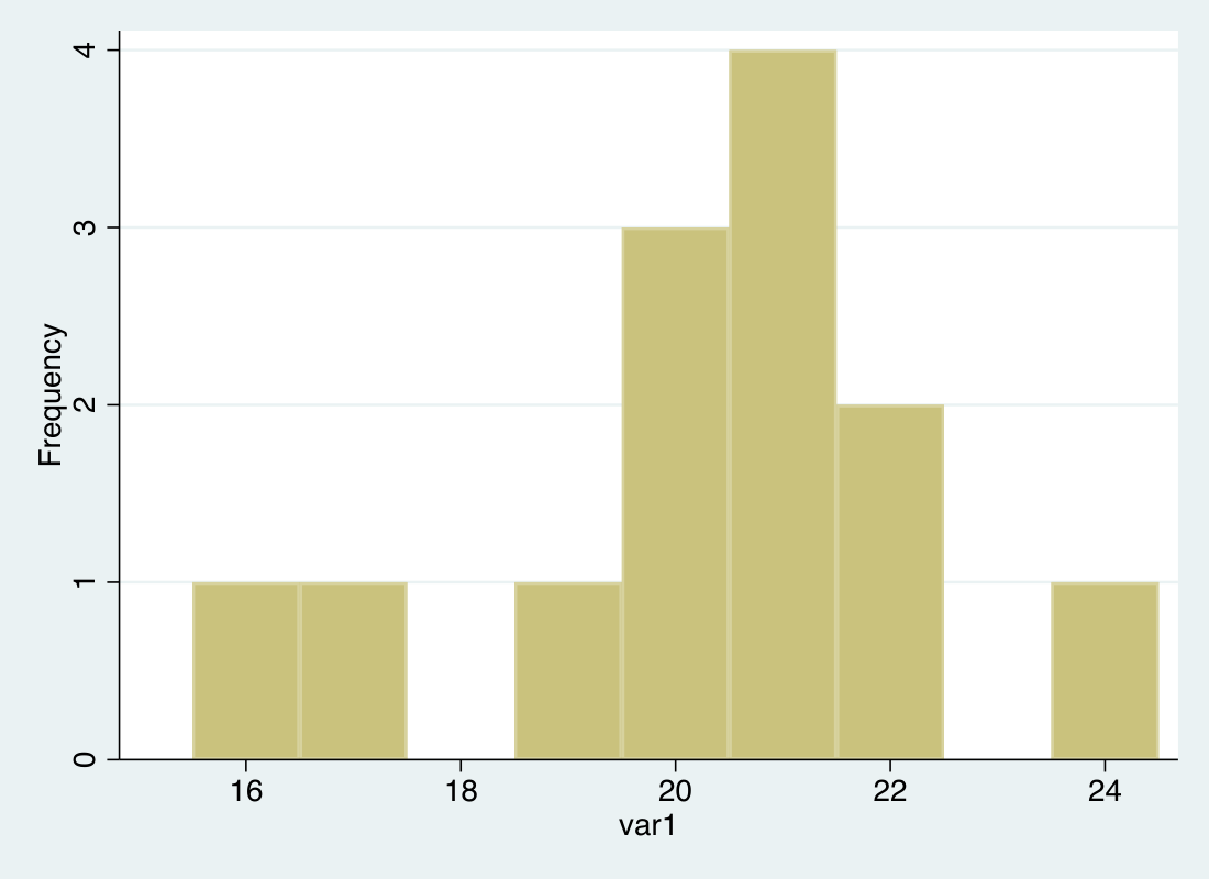
Suppose that for 13 households we have the following values for the variable Temperature:

\[21, 22, 17, 19, 20, 21, 20, 21, 21, 20, 24, 22, 16\]

The mode is 21, since this value occurs most often (four times)
To compute the median we first need to rank the values:

\[16, 17, 19,20,20, 20, \mathbf{21}, 21, 21, 21, 22, 22, 24\]

We compute the mean:

\[ \bar{X} = \frac{1}{13} (21+ 22+ 17+ 19+ 20+ 21+ 20+ 21+ 21+ 20+ 24+22+16) \approx 20.3 \]

Measures of spread

A common measure of spread is the standard deviation
It represents how much the values in our data typically deviate from the mean
The sample standard deviation is computed using the following formula:

$s$ = $\sqrt{\dfrac{1}{n-1}\displaystyle\sum_{i=1}^n (X_i-\bar{X})^2}$

Range: the difference between the largest and the smallest value in our data
Range and standard deviation are only sensible measures for interval/ratio variables

Distribution in the sample

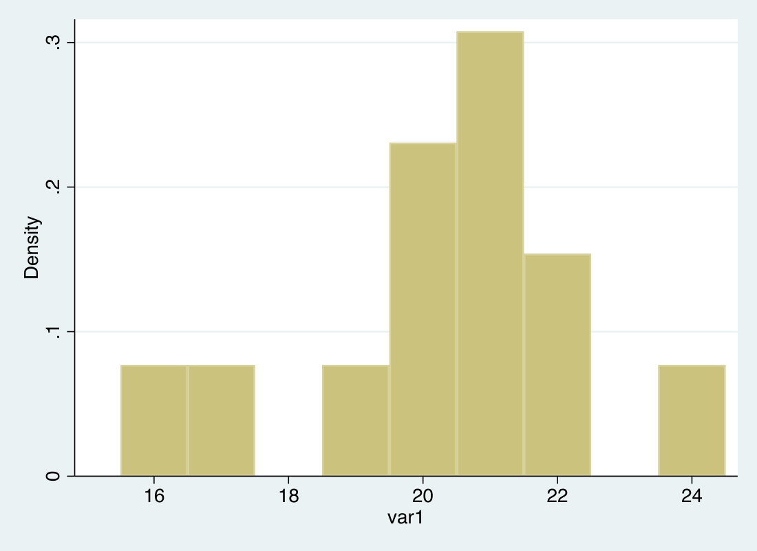
We can describe the distribution of the values of our variables using histograms
These describe how frequently (in relative or absolute terms) each value occurs in our data

Histogram
Data

Household	Temperature
1	21
2	22
3	17
4	19
5	20
6	21
7	20
8	21
9	21
10	20
11	24
12	22
13	16

Distribution in the sample

We can describe the distribution of the values of our variables using histograms
These describe how frequently (in relative or absolute terms) each value occurs in our data

Histogram
Data

Household	Temperature
1	21
2	22
3	17
4	19
5	20
6	21
7	20
8	21
9	21
10	20
11	24
12	22
13	16

Population mean and estimates

Quick recap: we want to say something about the variable $X$ = indoor temperature among Swedish households
Population mean, $\mu_X$: The average temperature in the population
We use the sample mean ($\bar{X}$) from our random sample as an estimate of the population mean
The sample mean from a random sample is probably not equal to the population mean
Due to chance we might “oversample” households whose indoor temperature is higher than average (or lower)

Random and systematic sampling error

Random sampling error: since the sample is random, the sample mean can differ from the population mean
Or we might make random measurement errors
The margin of error accounts for these deviations (more on this later)
Systematic sampling error: non-representative samples, e.g. due to non-response, or systematic measurement errors
Systematic sampling error is harder to do anything about

Illustration: random and systematic sampling error

100 fictional individuals by monthly income (thousands of SEK). Click a button to draw a random sample of 10 — point at (or tap) a figure to see their income

// One-time (non-reactive) global listener: on mobile, rotating the
// screen fires "orientationchange" while iOS Safari is still mid-way
// through animating the address bar/viewport, so reveal.js's own
// resize handler picks up transitional (wrong) dimensions and mis-
// scales the slide -- which is what made every interactive figure
// disappear until a full reload. Re-running reveal.js's own layout
// pass a moment after rotation, once the viewport has settled, fixes
// this without touching any figure's own code.
orientationRelayout = {
  window.addEventListener("orientationchange", () => {
    setTimeout(() => {
      if (typeof Reveal !== "undefined" && Reveal.layout) Reveal.layout();
    }, 400);
  });
  return null;
}

function mulberry32(seed) {
  return function () {
    seed |= 0; seed = (seed + 0x6D2B79F5) | 0;
    let t = Math.imul(seed ^ (seed >>> 15), 1 | seed);
    t = (t + Math.imul(t ^ (t >>> 7), 61 | t)) ^ t;
    return ((t ^ (t >>> 14)) >>> 0) / 4294967296;
  };
}

// Fixed seed so the "population" of 100 people is identical every time
// the slide loads (not re-randomized on each render) -- so everyone in
// the room is looking at the same μ and the same 100 individuals.
// Log-normal draw: right-skewed, mimics the rough shape of Sweden's
// income distribution (most people clustered in the middle, a long
// tail of high earners). Numbers are invented, not real statistics.
// Income is kept continuous (not rounded) so incomes essentially never
// collide exactly -- rounding to whole thousands created enough
// duplicate values to force a noticeably taller, blockier swarm than
// the underlying distribution actually has.
incomePopulation = {
  const rng = mulberry32(20260813);
  const people = [];
  for (let i = 0; i < 100; i++) {
    const u1 = rng(), u2 = rng();
    const z = Math.sqrt(-2 * Math.log(u1)) * Math.cos(2 * Math.PI * u2);
    const income = Math.exp(3.33 + 0.35 * z);
    people.push({ id: i + 1, income: Math.max(12, income) });
  }
  return people;
}

incomeMu = d3.mean(incomePopulation, d => d.income)

incomePlotWidth = 1100
incomeMarginLeft = 50
incomeMarginRight = 50
incomeRowHeight = 42
incomeFigSpacing = 18
incomeTopPad = 45

incomeXScale = d3.scaleLinear()
  .domain([d3.min(incomePopulation, d => d.income) - 2, d3.max(incomePopulation, d => d.income) + 2])
  .range([incomeMarginLeft, incomePlotWidth - incomeMarginRight])

// Beeswarm-style packing: sort by income, then stack each figure into
// the first row where it doesn't overlap the previous figure already
// placed in that row -- rows fill up densely where incomes cluster,
// so the swarm's shape roughly traces the underlying distribution.
incomeLayout = {
  const sorted = [...incomePopulation].sort((a, b) => a.income - b.income);
  const rowsLastX = [];
  const placed = [];
  for (const person of sorted) {
    const x = incomeXScale(person.income);
    let row = rowsLastX.findIndex(lastX => x - lastX >= incomeFigSpacing);
    if (row === -1) {
      row = rowsLastX.length;
      rowsLastX.push(x);
    } else {
      rowsLastX[row] = x;
    }
    placed.push({ ...person, x, row });
  }
  return placed;
}

incomeWeightRichBias = (d) => d.income
incomeWeightPoorBias = (d) => 1 / d.income
incomeWeightFlat = (d) => 1

function weightedSampleWithoutReplacement(items, weightFn, n) {
  const pool = items.map(d => ({ item: d, w: weightFn(d) }));
  const chosen = [];
  for (let k = 0; k < n && pool.length > 0; k++) {
    const total = d3.sum(pool, p => p.w);
    let r = Math.random() * total;
    let idx = 0;
    for (; idx < pool.length - 1; idx++) {
      r -= pool[idx].w;
      if (r <= 0) break;
    }
    chosen.push(pool[idx].item);
    pool.splice(idx, 1);
  }
  return chosen;
}

mutable incomeSample = null

html`<div class="sd-buttons-wrap"><div class="sd-buttons">
  ${Inputs.button("🎲 Fully random sample", {
    value: null,
    reduce: () => {
      const sample = weightedSampleWithoutReplacement(incomePopulation, incomeWeightFlat, 10);
      mutable incomeSample = { ids: new Set(sample.map(d => d.id)), xbar: d3.mean(sample, d => d.income), method: "Fully random sample" };
      return null;
    }
  })}
  ${Inputs.button("⬆️ Undersamples the poor", {
    value: null,
    reduce: () => {
      const sample = weightedSampleWithoutReplacement(incomePopulation, incomeWeightRichBias, 10);
      mutable incomeSample = { ids: new Set(sample.map(d => d.id)), xbar: d3.mean(sample, d => d.income), method: "Undersamples the poor (rich chosen more often)" };
      return null;
    }
  })}
  ${Inputs.button("⬇️ Undersamples the rich", {
    value: null,
    reduce: () => {
      const sample = weightedSampleWithoutReplacement(incomePopulation, incomeWeightPoorBias, 10);
      mutable incomeSample = { ids: new Set(sample.map(d => d.id)), xbar: d3.mean(sample, d => d.income), method: "Undersamples the rich (poor chosen more often)" };
      return null;
    }
  })}
  ${Inputs.button("↺", {
    value: null,
    reduce: () => { mutable incomeSample = null; return null; }
  })}
</div></div>`

// Whole SVG is rebuilt on every click (cheap at n=100) -- only the
// hover/click tooltip is kept out of the reactive graph (plain D3
// show/hide via closures), so hovering never triggers a rebuild. Once
// a figure is clicked (pinned), further hovering is ignored entirely
// until the user clicks empty space to unpin -- same locked-selection
// pattern used for the household dots on L2.
//
// Each figure gets its own invisible, generously-sized hit-circle
// (radius 17, well beyond the visible stick-figure's own thin lines)
// that pointer/click handlers are attached to instead of the visible
// shapes themselves -- otherwise the actual clickable area is only the
// handful of pixels covered by 2px-wide strokes, which is what made
// pointing feel overly sensitive before.
incomeSvgWrap = {
  const maxRow = d3.max(incomeLayout, d => d.row);
  const baseY = incomeTopPad + (maxRow + 1) * incomeRowHeight;
  const axisY = baseY + 10;
  const height = axisY + 32;

  const outer = d3.create("div").attr("class", "income-pop-wrap");
  const svg = outer.append("svg")
    .attr("viewBox", `0 0 ${incomePlotWidth} ${height}`)
    .attr("width", incomePlotWidth)
    .attr("height", height)
    .attr("class", "income-pop-svg");
  const tip = outer.append("div").attr("class", "income-tip").style("display", "none");

  let pinned = false;
  function showTip(node, text) {
    tip.text(text).style("display", "block");
    const wrapRect = outer.node().getBoundingClientRect();
    const nodeRect = node.getBoundingClientRect();
    const tipNode = tip.node();
    let left = (nodeRect.left - wrapRect.left) + nodeRect.width / 2 - tipNode.offsetWidth / 2;
    let top = (nodeRect.top - wrapRect.top) - tipNode.offsetHeight - 8;
    if (left < 0) left = 0;
    if (left + tipNode.offsetWidth > wrapRect.width) left = wrapRect.width - tipNode.offsetWidth;
    if (top < 0) top = (nodeRect.bottom - wrapRect.top) + 8;
    tip.style("left", `${left}px`).style("top", `${top}px`);
  }
  function hideTip() { if (!pinned) tip.style("display", "none"); }

  // Axis line + hand-drawn ticks (short mark rising from the baseline,
  // number beneath it), matching the convention used for every other
  // number-line plot in this deck.
  svg.append("line")
    .attr("x1", incomeMarginLeft).attr("x2", incomePlotWidth - incomeMarginRight)
    .attr("y1", axisY).attr("y2", axisY).attr("stroke", "#333").attr("stroke-width", 1);
  incomeXScale.ticks(10).forEach(t => {
    svg.append("line")
      .attr("x1", incomeXScale(t)).attr("x2", incomeXScale(t))
      .attr("y1", axisY).attr("y2", axisY + 5)
      .attr("stroke", "#333").attr("stroke-width", 1);
    svg.append("text")
      .attr("x", incomeXScale(t)).attr("y", axisY + 19)
      .attr("text-anchor", "middle").attr("font-size", 14).attr("fill", "#555")
      .text(t);
  });

  const muX = incomeXScale(incomeMu);
  svg.append("line")
    .attr("x1", muX).attr("x2", muX).attr("y1", 16).attr("y2", axisY)
    .attr("stroke", "#000").attr("stroke-width", 2.5).attr("stroke-dasharray", "7,4");
  svg.append("text")
    .attr("x", muX).attr("y", 13)
    .attr("text-anchor", "middle").attr("font-size", 17).attr("fill", "#000")
    .text(`μ = ${fmtNum(incomeMu, 1)}`);

  if (incomeSample) {
    const xbarX = incomeXScale(incomeSample.xbar);
    svg.append("line")
      .attr("x1", xbarX).attr("x2", xbarX).attr("y1", 16).attr("y2", axisY)
      .attr("stroke", "#dc2626").attr("stroke-width", 2.5);
    svg.append("text")
      .attr("x", xbarX).attr("y", height - 4)
      .attr("text-anchor", "middle").attr("font-size", 17).attr("fill", "#dc2626")
      .text(`X̄ = ${fmtNum(incomeSample.xbar, 1)}`);
  }

  // Legend
  svg.append("circle").attr("cx", incomePlotWidth - 110).attr("cy", 16).attr("r", 6).attr("fill", "#dc2626");
  svg.append("text").attr("x", incomePlotWidth - 98).attr("y", 21)
    .attr("font-size", 14).attr("fill", "#333").text("= in the sample");

  incomeLayout.forEach(d => {
    const g = svg.append("g")
      .attr("transform", `translate(${d.x}, ${baseY - d.row * incomeRowHeight})`)
      .style("cursor", "pointer");

    const sampled = incomeSample && incomeSample.ids.has(d.id);
    const color = sampled ? "#dc2626" : "#475569";

    // Soft halo behind sampled figures, in addition to the color swap
    // above -- makes the highlighted individuals unmistakable even from
    // the back of a lecture hall.
    if (sampled) {
      g.append("circle").attr("cy", -11).attr("r", 19).attr("fill", "rgba(220, 38, 38, 0.18)");
    }

    g.append("circle").attr("cy", -25).attr("r", 5).attr("fill", color);
    g.append("line").attr("x1", 0).attr("y1", -20).attr("x2", 0).attr("y2", -4).attr("stroke", color).attr("stroke-width", sampled ? 3 : 2);
    g.append("line").attr("x1", -6).attr("y1", -14).attr("x2", 6).attr("y2", -14).attr("stroke", color).attr("stroke-width", sampled ? 3 : 2);
    g.append("line").attr("x1", 0).attr("y1", -4).attr("x2", -6).attr("y2", 8).attr("stroke", color).attr("stroke-width", sampled ? 3 : 2);
    g.append("line").attr("x1", 0).attr("y1", -4).attr("x2", 6).attr("y2", 8).attr("stroke", color).attr("stroke-width", sampled ? 3 : 2);

    // Invisible, generously-sized hit target -- the actual pointer/click
    // handlers live here, not on the thin visible strokes above.
    const hit = g.append("circle")
      .attr("cy", -11).attr("r", 17)
      .attr("fill", "transparent")
      .style("pointer-events", "all");

    hit.on("pointerenter", (event) => {
      if (event.pointerType === "touch" || pinned) return;
      showTip(hit.node(), `Individual #${d.id}: ${fmtNum(d.income, 0)} thousand SEK/month`);
    })
    .on("pointerleave", (event) => {
      if (event.pointerType === "touch") return;
      hideTip();
    })
    .on("click", (event) => {
      pinned = true;
      showTip(hit.node(), `Individual #${d.id}: ${fmtNum(d.income, 0)} thousand SEK/month`);
      event.stopPropagation();
    });
  });

  svg.on("click", () => { pinned = false; tip.style("display", "none"); });

  return outer.node();
}

html`<div class="ojs-plot-wrap">
  ${incomeSvgWrap}
  <div class="ojs-plot-xlabel">Monthly income (thousands of SEK)</div>
</div>`

html`<div class="ci-demo-note" style="min-height: 2.4em;">${
  !incomeSample
    ? md`*Click one of the buttons above to draw a random sample of 10 individuals.*`
    : md`**${incomeSample.method}** — the sample mean is **X̄ = ${fmtNum(incomeSample.xbar, 1)}** thousand SEK, compared to the population mean **μ = ${fmtNum(incomeMu, 1)}** thousand SEK (difference: ${fmtNum(incomeSample.xbar - incomeMu, 1)} thousand SEK).`
}</div>`

How confident can we be?

Suppose we only have random sampling error; then the sample mean (our estimate) is not necessarily equal to the population mean
Example: we randomly select 2000 households and compute a sample mean of $\bar{X} = 18$
Our boss asks us to say something about the average indoor temperature among Swedish households — what should we answer?
In this particular sample we got $\bar{X} = 18$, so that’s our best “guess”, but how confident are we that the population mean isn’t, say, 17?
The sample mean we compute might, due to chance, differ from the population mean, so perhaps $\mu_{X} = 17$

An interval

What if we could present an interval symmetric around our estimate $\bar{X}$?
We say that we believe the true population mean lies between the lower and upper bounds of the interval
For example, 18 $\pm$ 3, i.e. that the true population mean is somewhere between 15 (18-3 = 15) and 21 (18+3 = 21)
We can then use the interval to dismiss (reject) claims that the average indoor temperature in the population is a value outside the interval
How do we decide how wide the interval should be? Is there a scientific method?

Random variables

To understand this method we first need to learn about the following concepts/ideas:
1. random variables,
2. probability distributions,
3. the sample mean is a random variable,
4. and has a known probability distribution,
5. which is (approximately) a normal distribution,
6. and has properties that help us determine the width of the interval
First and foremost, random variables: the values we observe are determined by random events
Example: the weather tomorrow at 9am; the value of a randomly drawn card from a deck
Or, the indoor temperature of a randomly chosen household that answers our survey

Random variables and probabilities

For many random variables, the different outcomes have different probabilities: some outcomes are more likely than others
Suppose we have a random variable that measures the age of the next person to walk into the lecture hall
Is it likely that a four-year-old walks in? Or that the person is between 20 and 40?
For this random variable it’s obvious that some outcomes, and thus values, are more likely than others

Probability distribution

A probability distribution shows how likely different values are to be observed (compare with a histogram)
The area under the curve between two points shows the probability that the random variable takes a value in between

// Log-normal, not the normal distribution -- students see the normal
// distribution formally a few slides later, so this generic example
// deliberately uses a differently-shaped (right-skewed) curve instead
// of previewing that exact shape here.
function logNormalPDF(x, mu, sigma) {
  if (x <= 0) return 0;
  return (1 / (x * sigma * Math.sqrt(2 * Math.PI))) * Math.exp(-((Math.log(x) - mu) ** 2) / (2 * sigma * sigma));
}

probMu = 3.3
probSigma = 0.5

probXDomain = [0, 100]

mutable probX = null

probPts = d3.range(probXDomain[0], probXDomain[1] + 0.1, 0.2).map(x => ({ x, y: logNormalPDF(x, probMu, probSigma) }))

// Trapezoidal-rule integration of the density from 0 to x, using the
// same fixed step as probPts so the shaded area and the printed
// probability are always consistent with each other.
function probCdfFrom0(x) {
  const step = 0.2;
  let area = 0;
  let prev = logNormalPDF(0, probMu, probSigma);
  for (let t = step; t <= x; t += step) {
    const cur = logNormalPDF(t, probMu, probSigma);
    area += (prev + cur) / 2 * step;
    prev = cur;
  }
  return area;
}

probPlotWidth = 860
probPlotHeight = 380
probMarginTop = 20
probMarginRight = 20
probMarginBottom = 40
probMarginLeft = 30
probYDomain = [-0.001, d3.max(probPts, d => d.y) * 1.15]

probMarks = {
  const m = [];
  if (probX !== null) {
    const shaded = probPts.filter(d => d.x <= probX);
    m.push(Plot.areaY(shaded, { x: "x", y: "y", fill: "#a855f7", fillOpacity: 0.35 }));
  }
  m.push(Plot.line(probPts, { x: "x", y: "y", stroke: "#2563eb", strokeWidth: 3 }));

  // Hand-drawn ticks (short mark rising from y=0, number beneath it)
  // instead of Plot's own axis, matching the convention used
  // throughout this deck.
  for (const t of d3.scaleLinear().domain(probXDomain).ticks(10)) {
    m.push(Plot.ruleX([{ x: t, y1: 0, y2: 0.0015 }], { x: "x", y1: "y1", y2: "y2", stroke: "#333", strokeWidth: 1 }));
    m.push(Plot.text([{ x: t, y: 0, label: String(t) }], { x: "x", y: "y", text: "label", dy: 14, fontSize: 13, fill: "#555" }));
  }

  if (probX !== null) {
    m.push(Plot.ruleX([{ x: probX, y1: 0, y2: logNormalPDF(probX, probMu, probSigma) }],
      { x: "x", y1: "y1", y2: "y2", stroke: "#7e22ce", strokeWidth: 2 }));
    m.push(Plot.text([{ x: probX, y: logNormalPDF(probX, probMu, probSigma), label: "x = " + fmtNum(probX, 1) }],
      { x: "x", y: "y", text: "label", dy: -10, fontSize: 14, fill: "#7e22ce" }));
  }
  m.push(Plot.ruleY([0], { stroke: "#333" }));
  return m;
}

// Transparent overlay rect for pointer capture: Plot's own event
// system only exposes marks directly under the cursor, not the raw
// pointer position, so a plain D3 rect layered on top (same x-scale
// and margins as the Plot figure below) reads the pointer's data-x
// value directly. A fresh class name (not .ojs-dots-overlay, which by
// convention is purely decorative and pointer-events: none) since this
// overlay is deliberately interactive.
probOverlay = {
  const xScale = d3.scaleLinear().domain(probXDomain).range([probMarginLeft, probPlotWidth - probMarginRight]);
  const svg = d3.create("svg")
    .attr("viewBox", `0 0 ${probPlotWidth} ${probPlotHeight}`)
    .attr("width", probPlotWidth)
    .attr("height", probPlotHeight)
    .attr("class", "ojs-click-overlay");

  svg.append("rect")
    .attr("x", probMarginLeft).attr("y", 0)
    .attr("width", probPlotWidth - probMarginLeft - probMarginRight)
    .attr("height", probPlotHeight)
    .attr("fill", "transparent")
    .style("cursor", "crosshair")
    .on("pointermove", (event) => {
      const [mx] = d3.pointer(event);
      mutable probX = Math.max(probXDomain[0], Math.min(probXDomain[1], xScale.invert(mx)));
    })
    .on("click", (event) => {
      const [mx] = d3.pointer(event);
      mutable probX = Math.max(probXDomain[0], Math.min(probXDomain[1], xScale.invert(mx)));
    });

  return svg.node();
}

html`<div class="ojs-plot-wrap">
  <div class="ojs-plot-overlay">
    ${Plot.plot({
      width: probPlotWidth,
      height: probPlotHeight,
      marginTop: probMarginTop,
      marginRight: probMarginRight,
      marginBottom: probMarginBottom,
      marginLeft: probMarginLeft,
      x: { domain: probXDomain, label: null, ticks: 0 },
      y: { domain: probYDomain, label: null, ticks: 0 },
      marks: probMarks
    })}
    ${probOverlay}
  </div>
  <div class="ojs-plot-xlabel">x</div>
</div>`

html`<div class="ci-demo-note" style="min-height: 2em;">${
  probX === null
    ? md`*Point or click under the curve to compute P(0 &lt; X &lt; x).*`
    : md`**P(0 &lt; X &lt; ${fmtNum(probX, 1)}) = ${fmtNum(probCdfFrom0(probX), 3)}**`
}</div>`

Example: probability distributions

Back to our scenario

All random variables follow a probability distribution
In most cases, however, we don’t know which probability distribution it is
The variable $X$ = indoor temperature is a random variable: we don’t know which value we’ll observe until we randomly select a household
We can define new random variables based on $X$ using mathematical operations
Example:
- $Y = X + 5$
- $Z = X_1 + X_2$
- $\bar{X} = (X_1 + X_2 + X_3 + X_4 + X_5)/5 \quad$ (=the sample mean)
$\bar{X}$ is therefore also a random variable — Visualization

The sample mean is a random variable

$\bar{X}$ is a random variable and therefore follows a probability distribution
Because $\bar{X}$ is computed from a sample, its probability distribution is called the sampling distribution
Quick summary:
- There’s a thing called random variables,
- all random variables have a probability distribution,
- the sample mean (from a random sample) is a random variable,
- and therefore follows a probability distribution (which we call the sampling distribution)
The Central Limit Theorem: the sampling distribution of the sample mean can be approximated by a normal distribution Simulation

Normal distribution

The normal distribution has a number of desirable properties
It is symmetric around its mean, $\mu$
The same probability of getting a value less than the mean $\mu$ as getting a value greater than the mean $\mu$
A normal distribution can be fully described by two parameters: the mean $\mu$ and the standard deviation $\sigma$
The mean $\mu$ determines the “center” of the distribution, while the standard deviation $\sigma$ describes the spread

Normal distribution: different $\mu$ and $\sigma$

For different values of the mean $\mu$ and the standard deviation $\sigma$, the normal distribution takes on a different location and shape

viewof mu = {
  const el = Inputs.range([80, 120], {value: 100, step: 1, label: "μ"});
  el.classList.add("small-slider");
  return el;
}

viewof sigma = {
  const el = Inputs.range([5, 20], {value: 10, step: 1, label: "σ"});
  el.classList.add("small-slider");
  return el;
}

normalPDF = (x, mu, sigma) =>
  (1 / (sigma * Math.sqrt(2 * Math.PI))) * Math.exp(-0.5 * ((x - mu) / sigma) ** 2)

function fmtNum(x, decimals = 2) {
  return x.toFixed(decimals);
}

pts = d3.range(30, 170, 0.5).map(x => ({x, y: normalPDF(x, mu, sigma)}))

marksMuSigma = {
  const m = [
    Plot.line(pts, { x: "x", y: "y", stroke: "#2563eb", strokeWidth: 3 }),
    Plot.ruleX([{ x: mu, y1: 0, y2: 0.085 }], { x: "x", y1: "y1", y2: "y2", stroke: "#666", strokeDasharray: "4,3" })
  ];
  // Hand-drawn ticks (short mark rising from y=0, number beneath it)
  // instead of Plot's own axis, which put its numbers too far below
  // the line.
  for (const t of d3.scaleLinear().domain([30, 170]).ticks(8)) {
    m.push(Plot.ruleX([{ x: t, y1: 0, y2: 0.003 }], { x: "x", y1: "y1", y2: "y2", stroke: "#333", strokeWidth: 1 }));
    m.push(Plot.text([{ x: t, y: 0, label: String(t) }], { x: "x", y: "y", text: "label", dy: 16, fontSize: 14, fill: "#555" }));
  }
  m.push(Plot.ruleY([0], { stroke: "#333" }));
  return m;
}

html`<div class="ojs-plot-wrap">
  ${Plot.plot({
    width: 860,
    height: 440,
    marginBottom: 46,
    marginLeft: 50,
    style: "font-size: 15px;",
    x: {domain: [30, 170], label: null, ticks: 0},
    y: {domain: [-0.005, 0.09], label: null},
    marks: marksMuSigma
  })}
  <div class="ojs-plot-xlabel">x</div>
</div>`

Probabilities in the normal distribution

The probability that a certain value is observed for a random variable that follows a normal distribution is shown in the graph below
For example, out of 100 trials, about 68 of them will take on a value between $\mu - \sigma$ and $\mu + \sigma$

mu1 = 100
sigma1 = 10

mutable sdLevel = 0

mutable simPoints = null

mutable numericExample = false

pts3 = d3.range(mu1 - 4 * sigma1, mu1 + 4 * sigma1, 0.1).map(x => ({ x, y: normalPDF(x, mu1, sigma1) }))

sdPlotWidth = 860
sdPlotHeight = 438
sdMarginTop = 20
sdMarginRight = 20
sdMarginBottom = 48
sdMarginLeft = 30
sdXDomain = [mu1 - 4.6 * sigma1, mu1 + 4.6 * sigma1]
sdYDomain = [-0.01, 0.09]

html`<div class="sd-buttons-wrap">
  <div class="sd-buttons-label">Show interval for:</div>
  <div class="sd-buttons">
    ${Inputs.button("σ", { value: null, reduce: () => { mutable sdLevel = 1; return null; } })}
    ${Inputs.button("2σ", { value: null, reduce: () => { mutable sdLevel = 2; return null; } })}
    ${Inputs.button("3σ", { value: null, reduce: () => { mutable sdLevel = 3; return null; } })}
    ${Inputs.button("🔢 Numeric example", {
      value: null,
      reduce: () => { mutable numericExample = !numericExample; return null; }
    })}
  </div>
  <div class="sd-buttons">
    ${Inputs.button("🎲 Simulate 100", {
      value: null,
      reduce: () => {
        mutable simPoints = {
          values: d3.range(100).map(() => mu1 + randNormal() * sigma1),
          delay: 20,
          duration: 900,
          radius: 4
        };
        return null;
      }
    })}
    ${Inputs.button("🎲 Simulate 1000", {
      value: null,
      reduce: () => {
        mutable simPoints = {
          values: d3.range(1000).map(() => mu1 + randNormal() * sigma1),
          delay: 3.5,
          duration: 900,
          radius: 2
        };
        return null;
      }
    })}
    ${Inputs.button("↺", {
      value: null,
      reduce: () => {
        mutable sdLevel = 0;
        mutable simPoints = null;
        return null;
      }
    })}
  </div>
</div>`

marksSd = {
  const m = [];
  const lo = mu1 - sdLevel * sigma1;
  const hi = mu1 + sdLevel * sigma1;
  if (sdLevel > 0) {
    const band = pts3.filter(d => d.x >= lo && d.x <= hi);
    m.push(Plot.areaY(band, { x: "x", y: "y", fill: "#a855f7", fillOpacity: 0.35 }));
  }
  m.push(Plot.line(pts3, { x: "x", y: "y", stroke: "#2563eb", strokeWidth: 3 }));
  m.push(Plot.ruleX([{ x: mu1, y1: 0, y2: normalPDF(mu1, mu1, sigma1) }],
    { x: "x", y1: "y1", y2: "y2", stroke: "#666", strokeDasharray: "4,3", strokeWidth: 1.5 }));
  m.push(Plot.text([{ x: mu1, y: 0, label: "μ" }], { x: "x", y: "y", text: "label", dy: 18, fontSize: 15 }));
  if (numericExample) {
    m.push(Plot.text([{ x: mu1, y: 0, label: `μ = ${mu1}` }],
      { x: "x", y: "y", text: "label", dy: 36, fontSize: 13, fill: "#000" }));
  }
  if (sdLevel > 0) {
    const sign = sdLevel === 1 ? "σ" : sdLevel + "σ";
    const pct = { 1: "68.27%", 2: "95.45%", 3: "99.73%" }[sdLevel];
    m.push(Plot.ruleX([{ x: lo, y1: 0, y2: normalPDF(lo, mu1, sigma1) }],
      { x: "x", y1: "y1", y2: "y2", stroke: "#7e22ce", strokeWidth: 1 }));
    m.push(Plot.ruleX([{ x: hi, y1: 0, y2: normalPDF(hi, mu1, sigma1) }],
      { x: "x", y1: "y1", y2: "y2", stroke: "#7e22ce", strokeWidth: 1 }));
    m.push(Plot.text([{ x: lo, y: 0, label: "μ − " + sign }],
      { x: "x", y: "y", text: "label", dy: 18, fontSize: 14, fill: "#7e22ce" }));
    m.push(Plot.text([{ x: hi, y: 0, label: "μ + " + sign }],
      { x: "x", y: "y", text: "label", dy: 18, fontSize: 14, fill: "#7e22ce" }));
    m.push(Plot.text([{ x: mu1, y: normalPDF(mu1, mu1, sigma1), label: pct }],
      { x: "x", y: "y", text: "label", dy: -10, fontSize: 16, fill: "#7e22ce" }));
    if (numericExample) {
      const delta = sdLevel * sigma1;
      m.push(Plot.text([{ x: lo, y: 0, label: `μ − ${sign} = ${mu1} − ${delta} = ${lo}` }],
        { x: "x", y: "y", text: "label", dy: 36, fontSize: 13, fill: "#7e22ce" }));
      m.push(Plot.text([{ x: hi, y: 0, label: `μ + ${sign} = ${mu1} + ${delta} = ${hi}` }],
        { x: "x", y: "y", text: "label", dy: 36, fontSize: 13, fill: "#7e22ce" }));
    }
  }
  m.push(Plot.ruleY([0], { stroke: "#333" }));
  return m;
}

// Falling-dots overlay: built with raw D3 (not Observable Plot), using
// our own linear scale that matches the Plot figure's own domain and
// pixel margins exactly, so dots land at the right x-position on the
// axis. Kept as a *separate* SVG layered on top of the Plot figure via
// CSS, so it only depends on simPoints -- switching σ/2σ/3σ afterwards
// never re-triggers the fall animation or disturbs the dots.
dotsOverlay = {
  const xScale = d3.scaleLinear().domain(sdXDomain).range([sdMarginLeft, sdPlotWidth - sdMarginRight]);
  // The y-domain's minimum is -0.01, not 0 (there's a sliver of
  // padding below the axis), so "where y=0 sits" is NOT simply the
  // bottom margin -- it has to go through the same scale Plot itself
  // uses, otherwise the dots land below the visible axis rule.
  const yScale = d3.scaleLinear().domain(sdYDomain).range([sdPlotHeight - sdMarginBottom, sdMarginTop]);
  const svg = d3.create("svg")
    .attr("viewBox", `0 0 ${sdPlotWidth} ${sdPlotHeight}`)
    .attr("width", sdPlotWidth)
    .attr("height", sdPlotHeight)
    .attr("class", "ojs-dots-overlay");

  if (simPoints) {
    const axisY = yScale(0);
    const topY = sdMarginTop;
    svg.selectAll("circle")
      .data(simPoints.values)
      .join("circle")
      .attr("cx", d => xScale(d))
      .attr("cy", topY)
      .attr("r", simPoints.radius)
      .attr("fill", "#dc2626")
      .attr("fill-opacity", 0.7)
      .transition()
      .delay((d, i) => i * simPoints.delay)
      .duration(simPoints.duration)
      .ease(d3.easeCubicIn)
      .attr("cy", axisY);
  }

  return svg.node();
}

html`<div class="ojs-plot-wrap">
  <div class="ojs-plot-overlay">
    ${Plot.plot({
      width: sdPlotWidth,
      height: sdPlotHeight,
      marginTop: sdMarginTop,
      marginRight: sdMarginRight,
      marginBottom: sdMarginBottom,
      marginLeft: sdMarginLeft,
      x: { domain: sdXDomain, label: null, ticks: 0 },
      y: { domain: [-0.01, 0.09], label: null, ticks: 0 },
      marks: marksSd
    })}
    ${dotsOverlay}
  </div>
  <div class="ojs-plot-xlabel">x</div>
</div>`

html`<div class="ci-demo-note">${
  !simPoints
    ? ""
    : sdLevel === 0
      ? md`*Choose an interval (σ, 2σ, or 3σ) above to see how many of the ${simPoints.values.length} simulated observations fall inside it.*`
      : (() => {
          const lo = mu1 - sdLevel * sigma1, hi = mu1 + sdLevel * sigma1;
          const n = simPoints.values.length;
          const count = simPoints.values.filter(v => v >= lo && v <= hi).length;
          const sign = sdLevel === 1 ? "σ" : sdLevel + "σ";
          return md`**${count}** out of ${n} simulated observations (**${fmtNum(100 * count / n, 1)}%**) fell within **${sign}** of the mean.`;
        })()
}</div>`

Example: pizza delivery

Suppose the time it takes for an ordered pizza to be delivered follows a normal distribution with mean $\mu = 30$ minutes and standard deviation $\sigma = 5$ minutes
Each button press below simulates a single order: a pizza is randomly drawn and “lands” on the number line at its delivery time

muP = 30
sigmaP = 5

mutable sdLevelP = 0

mutable pizzaHistory = []

ptsP = d3.range(muP - 4.6 * sigmaP, muP + 4.6 * sigmaP, 0.1).map(x => ({ x, y: normalPDF(x, muP, sigmaP) }))

pPlotWidth = 860
pPlotHeight = 420
pMarginTop = 20
pMarginRight = 20
pMarginBottom = 50
pMarginLeft = 30
pXDomain = [muP - 4.6 * sigmaP, muP + 4.6 * sigmaP]
pYDomain = [-0.005, 0.09]
pBinWidth = 0.1

html`<div class="sd-buttons-wrap">
  <div class="sd-buttons-label">Show interval for:</div>
  <div class="sd-buttons">
    ${Inputs.button("σ", { value: null, reduce: () => { mutable sdLevelP = 1; return null; } })}
    ${Inputs.button("2σ", { value: null, reduce: () => { mutable sdLevelP = 2; return null; } })}
    ${Inputs.button("3σ", { value: null, reduce: () => { mutable sdLevelP = 3; return null; } })}
  </div>
  <div class="sd-buttons">
    ${Inputs.button("🍕 Order pizza", {
      value: null,
      reduce: () => {
        mutable pizzaHistory = [...pizzaHistory, muP + randNormal() * sigmaP];
        return null;
      }
    })}
    ${Inputs.button("↺", {
      value: null,
      reduce: () => {
        mutable sdLevelP = 0;
        mutable pizzaHistory = [];
        return null;
      }
    })}
  </div>
</div>`

marksP = {
  const m = [];
  const lo = muP - sdLevelP * sigmaP;
  const hi = muP + sdLevelP * sigmaP;
  if (sdLevelP > 0) {
    const band = ptsP.filter(d => d.x >= lo && d.x <= hi);
    m.push(Plot.areaY(band, { x: "x", y: "y", fill: "#a855f7", fillOpacity: 0.35 }));
  }
  m.push(Plot.line(ptsP, { x: "x", y: "y", stroke: "#2563eb", strokeWidth: 3 }));

  // Plot's own axis put its tick numbers too far below the number
  // line, so it's suppressed (ticks: 0 below) and drawn by hand here
  // instead: a short mark rising from y=0, number directly beneath it.
  for (const t of d3.scaleLinear().domain(pXDomain).ticks(8)) {
    m.push(Plot.ruleX([{ x: t, y1: 0, y2: 0.003 }],
      { x: "x", y1: "y1", y2: "y2", stroke: "#333", strokeWidth: 1 }));
    m.push(Plot.text([{ x: t, y: 0, label: String(t) }],
      { x: "x", y: "y", text: "label", dy: 14, fontSize: 14, fill: "#555" }));
  }

  m.push(Plot.ruleX([{ x: muP, y1: 0, y2: normalPDF(muP, muP, sigmaP) }],
    { x: "x", y1: "y1", y2: "y2", stroke: "#666", strokeDasharray: "4,3", strokeWidth: 1.5 }));
  if (sdLevelP > 0) {
    const pct = { 1: "68.27%", 2: "95.45%", 3: "99.73%" }[sdLevelP];
    m.push(Plot.ruleX([{ x: lo, y1: 0, y2: normalPDF(lo, muP, sigmaP) }],
      { x: "x", y1: "y1", y2: "y2", stroke: "#7e22ce", strokeWidth: 1 }));
    m.push(Plot.ruleX([{ x: hi, y1: 0, y2: normalPDF(hi, muP, sigmaP) }],
      { x: "x", y1: "y1", y2: "y2", stroke: "#7e22ce", strokeWidth: 1 }));
    m.push(Plot.text([{ x: muP, y: normalPDF(muP, muP, sigmaP), label: pct }],
      { x: "x", y: "y", text: "label", dy: -10, fontSize: 16, fill: "#7e22ce" }));
  }
  m.push(Plot.ruleY([0], { stroke: "#333" }));
  return m;
}

// Growing dot-histogram of past pizza deliveries: each order stacks a
// new dot on top of previous ones that landed in the same time-bin.
// Only the newest dot animates falling -- earlier ones are drawn
// directly in their already-landed stacked position, so re-ordering
// doesn't replay the whole history's animation every time.
pizzaOverlay = {
  const xScale = d3.scaleLinear().domain(pXDomain).range([pMarginLeft, pPlotWidth - pMarginRight]);
  const yScale = d3.scaleLinear().domain(pYDomain).range([pPlotHeight - pMarginBottom, pMarginTop]);
  const axisY = yScale(0);
  const dotR = 5;
  const step = 2 * dotR + 1;

  const svg = d3.create("svg")
    .attr("viewBox", `0 0 ${pPlotWidth} ${pPlotHeight}`)
    .attr("width", pPlotWidth)
    .attr("height", pPlotHeight)
    .attr("class", "ojs-dots-overlay");

  // Stack dots on the exact value, rounded to one decimal -- the same
  // precision the delivery time itself is displayed at -- rather than
  // a wider bin, so two orders only stack when they actually rounded
  // to the same tenth of a minute.
  const roundOf = v => Math.round(v / pBinWidth) * pBinWidth;
  const seenPerValue = new Map();
  const placed = pizzaHistory.map(v => {
    const r = roundOf(v).toFixed(1);
    const stackIndex = seenPerValue.get(r) ?? 0;
    seenPerValue.set(r, stackIndex + 1);
    const cx = xScale(Number(r));
    const cy = axisY - stackIndex * step - dotR;
    return { cx, cy };
  });

  svg.selectAll("circle")
    .data(placed)
    .join("circle")
    .attr("cx", d => d.cx)
    .attr("cy", (d, i) => i === placed.length - 1 ? pMarginTop : d.cy)
    .attr("r", dotR)
    .attr("fill", "#dc2626")
    .attr("fill-opacity", 0.8)
    .each(function (d, i) {
      if (i === placed.length - 1) {
        d3.select(this).transition().duration(700).ease(d3.easeCubicIn).attr("cy", d.cy);
      }
    });

  return svg.node();
}

html`<div class="ojs-plot-wrap">
  <div class="ojs-plot-overlay">
    ${Plot.plot({
      width: pPlotWidth,
      height: pPlotHeight,
      marginTop: pMarginTop,
      marginRight: pMarginRight,
      marginBottom: pMarginBottom,
      marginLeft: pMarginLeft,
      style: "font-size: 15px;",
      x: { domain: pXDomain, label: "Minutes", ticks: 0 },
      y: { domain: pYDomain, label: null, ticks: 0 },
      marks: marksP
    })}
    ${pizzaOverlay}
  </div>
</div>`

html`<div class="ci-demo-note">${
  pizzaHistory.length === 0
    ? md`*Click "Order pizza" to simulate a delivery time. Feel free to choose an interval (σ, 2σ, or 3σ) first.*`
    : (() => {
        const n = pizzaHistory.length;
        const last = pizzaHistory[n - 1];
        const lastLine = `Your latest pizza arrived after **${fmtNum(last, 1)}** minutes.`;
        if (sdLevelP === 0) return md`${lastLine} You have ordered **${n}** ${n === 1 ? "pizza" : "pizzas"} in total.`;
        const lo = muP - sdLevelP * sigmaP, hi = muP + sdLevelP * sigmaP;
        const count = pizzaHistory.filter(v => v >= lo && v <= hi).length;
        const sign = sdLevelP === 1 ? "σ" : sdLevelP + "σ";
        return md`${lastLine} You have ordered **${n}** ${n === 1 ? "pizza" : "pizzas"} in total, of which **${count}** (**${fmtNum(100 * count / n, 1)}%**) arrived within **${sign}** of the mean.`;
      })()
}</div>`

$\bar{X}$ (roughly) follows a normal distribution

Again: the Central Limit Theorem shows that the sample mean (roughly) follows a normal distribution
Moreover, we know that $\bar{X}$ for the random variable $X$ computed from our sample comes from a normal distribution whose $\mu$ equals the population mean of $X$
But we don’t know the values of $\mu$ or $\sigma$ (called the standard error in a sampling distribution)
We do know, however, that about 95 percent of all possible random samples will give a sample mean within the interval $\mu - 2 \times \sigma$ and $\mu + 2 \times \sigma$

Confidence interval

If we draw 100 random samples, 95 of them will give us a sample mean $\bar{X}$ within the interval $\mu - 2 \times \sigma$ and $\mu + 2 \times \sigma$ (symmetric around $\mu$)
We don’t know the value of $\sigma$, though; but what if we could estimate it?
Then we’d know the “width” of the interval around the mean $\mu$ that covers 95 out of 100 of the sample means
Remember the goal: present an estimate of the population mean together with an interval of plausible values
If the $\bar{X}$ we compute falls within that interval around $\mu$, then $\mu$ must also fall within a similar interval around our $\bar{X}$

Does the interval cover $\mu$?

The shaded area covers $\mu \pm 2\sigma$, that is, 95.45% of all realizations of $\bar{X}$ that fall closest to $\mu$. Draw a sample mean $\bar{X}$ to see whether an equally wide interval around $\bar{X}$ covers $\mu$

mu0 = 20
sigma0 = 2

function randNormal() {
  const u1 = Math.random(), u2 = Math.random();
  return Math.sqrt(-2 * Math.log(u1)) * Math.cos(2 * Math.PI * u2);
}

mutable draw = null

html`<div class="dice-rows">
  ${Inputs.button("🎲", {
    value: null,
    reduce: () => {
      let z;
      do { z = randNormal(); } while (Math.abs(z) >= 2);
      mutable draw = { x: mu0 + z * sigma0, inside: true };
      return null;
    }
  })}
  <span>Draw a realization: <strong>inside</strong> the 95% interval</span>
  ${Inputs.button("🎲", {
    value: null,
    reduce: () => {
      let z;
      do { z = randNormal(); } while (Math.abs(z) < 2);
      mutable draw = { x: mu0 + z * sigma0, inside: false };
      return null;
    }
  })}
  <span>Draw a realization: <strong>outside</strong> the 95% interval</span>
  ${Inputs.button("🎲", {
    value: null,
    reduce: () => {
      const z = randNormal();
      mutable draw = { x: mu0 + z * sigma0, inside: Math.abs(z) < 2 };
      return null;
    }
  })}
  <span>Draw a realization: completely at random</span>
  ${Inputs.button("↺", {
    value: null,
    reduce: () => {
      mutable draw = null;
      return null;
    }
  })}
  <span>Remove the realization (start over)</span>
</div>`

pts2 = d3.range(mu0 - 4 * sigma0, mu0 + 4 * sigma0, 0.05)
  .map(x => ({ x, y: normalPDF(x, mu0, sigma0) }))

marks = {
  const m = [];
  const bandPts = pts2.filter(d => d.x >= mu0 - 2 * sigma0 && d.x <= mu0 + 2 * sigma0);
  m.push(Plot.areaY(bandPts, { x: "x", y: "y", fill: "#a855f7", fillOpacity: 0.35 }));
  m.push(Plot.line(pts2, { x: "x", y: "y", stroke: "#2563eb", strokeWidth: 3 }));
  m.push(Plot.ruleX([{ x: mu0, y1: 0, y2: 0.22 }], { x: "x", y1: "y1", y2: "y2", stroke: "#000", strokeWidth: 2, strokeDasharray: "6,4" }));

  // Hand-drawn ticks (short mark rising from y=0, number beneath it)
  // instead of Plot's own axis, which put its numbers too far below
  // the line.
  for (const t of d3.scaleLinear().domain([mu0 - 4 * sigma0, mu0 + 4 * sigma0]).ticks(8)) {
    m.push(Plot.ruleX([{ x: t, y1: 0, y2: 0.008 }], { x: "x", y1: "y1", y2: "y2", stroke: "#333", strokeWidth: 1 }));
    m.push(Plot.text([{ x: t, y: 0, label: String(t) }], { x: "x", y: "y", text: "label", dy: 14, fontSize: 11, fill: "#555" }));
  }

  m.push(Plot.text([{ x: mu0, y: 0, label: "μ = 20" }], { x: "x", y: "y", text: "label", dy: 32, fontSize: 13, fill: "#000" }));
  if (draw) {
    const col = draw.inside ? "#dc2626" : "#f59e0b";
    m.push(Plot.link([{ x1: draw.x - 2 * sigma0, x2: draw.x + 2 * sigma0, y1: 0.06, y2: 0.06 }],
      { x1: "x1", x2: "x2", y1: "y1", y2: "y2", stroke: col, strokeWidth: 4 }));
    m.push(Plot.ruleX([{ x: draw.x, y1: 0, y2: 0.06 }],
      { x: "x", y1: "y1", y2: "y2", stroke: col, strokeWidth: 1 }));
    m.push(Plot.dot([{ x: draw.x, y: 0 }], { x: "x", y: "y", r: 6, fill: col }));
    m.push(Plot.text([{ x: draw.x, y: 0.06, label: "X̄ = " + fmtNum(draw.x, 2) }],
      { x: "x", y: "y", text: "label", dy: -10, fontSize: 15, fill: col }));
  }
  m.push(Plot.ruleY([0], { stroke: "#333" }));
  return m;
}

html`<div class="ojs-plot-row">
  <div class="ojs-plot-wrap">
    ${Plot.plot({
      width: 620,
      height: 300,
      marginBottom: 52,
      marginLeft: 50,
      x: { domain: [mu0 - 4 * sigma0, mu0 + 4 * sigma0], label: null, ticks: 0 },
      y: { domain: [-0.02, 0.24], label: null, ticks: 0 },
      marks: marks
    })}
    <div class="ojs-plot-xlabel">x</div>
  </div>
  <div class="ojs-plot-caption">
    95% interval<br>
    [μ − 2σ, μ + 2σ]<br>
    = [${mu0 - 2 * sigma0}, ${mu0 + 2 * sigma0}]
  </div>
</div>`

html`<div class="ci-demo-note">${
  draw
    ? (() => {
        const lo = fmtNum(draw.x - 2 * sigma0, 2), hi = fmtNum(draw.x + 2 * sigma0, 2);
        return draw.inside
          ? md`✅ This X̄ (= ${fmtNum(draw.x, 2)}) is one of the **95.45%** of realizations that fall within 2σ of μ. An equally wide interval, i.e. [${lo}, ${hi}], around this X̄ therefore covers the true μ.`
          : md`❌ This X̄ (= ${fmtNum(draw.x, 2)}) is one of the **4.55%** of realizations that fall *outside* 2σ of μ. An equally wide interval, i.e. [${lo}, ${hi}], around this X̄ therefore does **not** cover the true μ.`;
      })()
    : md`*Click one of the buttons above to draw a sample mean.*`
}</div>`

Using confidence intervals

$\bar{X}$ is our best guess of what the population mean, $\mu_X$, is
We believe our confidence interval covers $\mu_X$, i.e. that $\mu_X$ is equal to some value within the interval
What can we actually say about $\mu_X$?
If someone claims that $\mu_X = 25$: if our confidence interval does not cover 25, we do not believe $\mu_X$ can equal 25
If the confidence interval covers 25, we could not rule out that $\mu_X = 25$

How confident are we? Confidence level

Are we completely certain that our interval around $\bar{X}$ covers the true population mean?
In 95 out of 100 cases the sample will give a sample mean ($\bar{X}$) that lies within that interval around the population mean — but what about the remaining 5 cases?
We call the interval a 95 percent confidence interval
We can’t know whether our particular $\bar{X}$ is one of the 95 that fall within the interval, but it’s quite likely to be the case (95% chance)
The width of the confidence interval determines how confident we want to be when we claim to cover the true population mean

Confidence level and interval width

Draw a sample mean $\bar{X}$ and try 90%, 95%, and 99% confidence level — see how the interval gets wider the more confident you want to be

mutable ciDraw = null

mutable ciLevel = 0

html`<div class="sd-buttons-wrap">
  <div class="sd-buttons">
    ${Inputs.button("🎲 Draw X̄", {
      value: null,
      reduce: () => { mutable ciDraw = mu0 + randNormal() * sigma0; return null; }
    })}
    ${Inputs.button("90% CI", { value: null, reduce: () => { mutable ciLevel = 90; return null; } })}
    ${Inputs.button("95% CI", { value: null, reduce: () => { mutable ciLevel = 95; return null; } })}
    ${Inputs.button("99% CI", { value: null, reduce: () => { mutable ciLevel = 99; return null; } })}
    ${Inputs.button("↺", {
      value: null,
      reduce: () => { mutable ciDraw = null; mutable ciLevel = 0; return null; }
    })}
  </div>
</div>`

ciHypothesis = 26

ciXDomain = [mu0 - 4 * sigma0, mu0 + 4 * sigma0]

marksCI = {
  const m = [];
  const center = ciDraw ?? mu0;
  m.push(Plot.line(pts2, { x: "x", y: "y", stroke: "#2563eb", strokeWidth: 3 }));

  // Plot's own implicit x-axis wouldn't put its ticks/labels exactly
  // where we wanted (they kept landing well below the number line
  // instead of hugging it), so the axis is fully suppressed (see the
  // Plot.plot call below) and every tick here is drawn by hand as a
  // short mark rising *from* y=0, with its number directly beneath.
  for (const t of d3.scaleLinear().domain(ciXDomain).ticks(8)) {
    m.push(Plot.ruleX([{ x: t, y1: 0, y2: 0.012 }],
      { x: "x", y1: "y1", y2: "y2", stroke: "#333", strokeWidth: 1 }));
    m.push(Plot.text([{ x: t, y: 0, label: String(t) }],
      { x: "x", y: "y", text: "label", dy: 14, fontSize: 11, fill: "#555" }));
  }

  m.push(Plot.ruleX([{ x: mu0, y1: 0, y2: 0.22 }],
    { x: "x", y1: "y1", y2: "y2", stroke: "#666", strokeDasharray: "4,3" }));
  m.push(Plot.ruleX([{ x: ciHypothesis, y1: 0, y2: 0.22 }],
    { x: "x", y1: "y1", y2: "y2", stroke: "#f59e0b", strokeDasharray: "2,3", strokeWidth: 1.5 }));
  m.push(Plot.text([{ x: mu0, y: 0, label: `μ = ${mu0}` }],
    { x: "x", y: "y", text: "label", dy: 30, fontSize: 12, fill: "#666" }));
  m.push(Plot.text([{ x: ciHypothesis, y: 0, label: `claimed value: ${ciHypothesis}` }],
    { x: "x", y: "y", text: "label", dy: 30, fontSize: 12, fill: "#b45309" }));
  if (ciLevel > 0) {
    const tVal = { 90: 1.65, 95: 1.96, 99: 2.58 }[ciLevel];
    const lo = center - tVal * sigma0, hi = center + tVal * sigma0;
    m.push(Plot.link([{ x1: lo, x2: hi, y1: 0.06, y2: 0.06 }],
      { x1: "x1", x2: "x2", y1: "y1", y2: "y2", stroke: "#a855f7", strokeWidth: 5 }));
    if (ciDraw !== null) {
      m.push(Plot.ruleX([{ x: center, y1: 0, y2: 0.06 }],
        { x: "x", y1: "y1", y2: "y2", stroke: "#a855f7", strokeWidth: 1 }));
    }
    m.push(Plot.text([{ x: center, y: 0.06, label: `${ciLevel}% CI: [${fmtNum(lo, 2)}, ${fmtNum(hi, 2)}]  (t = ${fmtNum(tVal, 2)})` }],
      { x: "x", y: "y", text: "label", dy: -10, fontSize: 14, fill: "#7e22ce" }));
  }
  if (ciDraw !== null) {
    m.push(Plot.dot([{ x: ciDraw, y: 0 }], { x: "x", y: "y", r: 6, fill: "#dc2626" }));
    m.push(Plot.text([{ x: ciDraw, y: 0, label: `X̄ = ${fmtNum(ciDraw, 2)}` }],
      { x: "x", y: "y", text: "label", dy: 44, fontSize: 12, fill: "#dc2626" }));
  }
  m.push(Plot.ruleY([0], { stroke: "#333" }));
  return m;
}

html`<div class="ojs-plot-wrap">
  ${Plot.plot({
    width: 680,
    height: 300,
    marginBottom: 58,
    marginLeft: 50,
    x: { domain: ciXDomain, label: null, ticks: 0 },
    y: { domain: [-0.02, 0.24], label: null, ticks: 0 },
    marks: marksCI
  })}
  <div class="ojs-plot-xlabel">x</div>
</div>`

html`<div class="ci-demo-note" style="min-height: 6em;">${
  (ciDraw === null || ciLevel === 0)
    ? md`*Draw an X̄ and choose a confidence level (90%, 95%, or 99%) to see the confidence interval and the conclusion.*`
    : (() => {
        const tVal = { 90: 1.65, 95: 1.96, 99: 2.58 }[ciLevel];
        const lo = ciDraw - tVal * sigma0, hi = ciDraw + tVal * sigma0;
        const coversMu = lo <= mu0 && mu0 <= hi;
        const coversHyp = lo <= ciHypothesis && ciHypothesis <= hi;
        return md`For X̄ = **${fmtNum(ciDraw, 2)}**, a **${ciLevel}%** confidence interval runs from **${fmtNum(lo, 2)}** to **${fmtNum(hi, 2)}**. That interval **${coversMu ? "covers" : "does not cover"}** the true population value. It also **${coversHyp ? "covers" : "does not cover"}** the claimed mean of ${ciHypothesis}, which means that, with this confidence interval, we **${coversHyp ? "cannot rule out" : "can rule out"}** that ${ciHypothesis} is the mean.`;
      })()
}</div>`

Calculating a confidence interval

Remember that we don’t know the value of $\sigma$, but there’s a way to estimate it:

\[ \mbox{Estimate of } \sigma = \hat{\sigma} = \frac{s_X}{\sqrt{n}} \]

$s_X$ is the sample standard deviation for the variable $X$, and $n$ is the sample size
The confidence interval is computed using the following formula:

\[ \bar{X} \pm t \times \frac{s_X}{\sqrt{n}} \]

The $t$-value determines how wide the confidence interval should be

Calculating a confidence interval: example

Example: We measure the height of 10 randomly selected students at SU and compute the sample mean $\bar{X} = 171$
We know that estimated sample means follow a normal distribution with some $\mu_X$ and $\sigma$
We don’t know $\mu_X$, though — our best guess is $\bar{X}$
Suppose someone claims that the mean height among the students in the population equals 185
Could that really be true, given that we computed $\bar{X} = 171$ for our sample?

Does the confidence interval cover it?

We compute a confidence interval for our estimate and compare it with the value 185
First we decide on the confidence level
The more confident we want to be, the wider our confidence interval becomes
Suppose a 95% confidence interval covers 185
We cannot reject the claim (hypothesis) that $\bar{X}$ comes from a population where the mean is 185
In other words: these 10 students may well come from a population where the mean height is 185

Does the confidence interval not cover it?

Suppose the confidence interval does not cover 185
We can then, with 95% confidence, say that $\bar{X}$ does not come from a population where the mean is 185
Why? Well, our interval covers the true population mean, and if the interval does not cover 185, then 185 cannot be the true population mean
We conclude that these 10 students do not come from a population where the mean height is 185
Note: this doesn’t necessarily mean that the true population mean equals 171 Worked example

Statistical significance

Confidence intervals are related to statistical significance
In our example we asked whether the difference between our estimated mean and 185 is statistically significant
Statistical inference means that we compare our estimate with another value
If the confidence interval covers a value, $a$, we say that the difference between our estimate and $a$ is not statistically significant
This is also commonly described as the difference being “within the margin of error”

One more example

The week before the election, your friend claims that the Liberal Party (L) won’t get enough votes to clear the parliamentary threshold
Your friend points to a survey of 1900 respondents, in which L got 3.6% of the votes
Assume the survey was based on a random sample
We want to test whether the estimated mean (3.6%) comes from a population in which L gets 4% of voters’ votes
If so, we cannot rule out that L would currently clear the threshold, despite the survey result
We therefore construct a confidence interval for the estimated mean of 0.036 (expressed as a proportion)

Statistical inference

We use the formula:

\[ \bar{X} \pm t \times \frac{s}{\sqrt{n}}, \quad \mbox{or} \quad \bar{X} \pm t \times \sqrt{\frac{s^2}{n}} \]

$\bar{X}$ equals 0.036 and $n = 1900$
$s^2$ is the sample variance for $X$, obtained by computing $p(1-p)$, where $p$ is the share who vote for L in the sample (i.e. 0.036)
We compute a 95% confidence interval, so $t = 1.96$

\[ 0.036 \pm 1.96 \times \sqrt{\frac{(0.036\times(1-0.036))}{1900}} \]

The confidence interval is [0.028, 0.044], which covers 0.04

Simulation: the Central Limit Theorem

$X$ follows a Gamma distribution with population mean $\mu = 7$

cltMu = 7
cltShape = 3
cltRate = cltShape / cltMu
// 30, not more: this is deliberately right at the common "n ≥ 30 gives
// a reasonably normal-looking sampling distribution" rule of thumb --
// with n=100 the sampling distribution of X̄ was so narrow the spread
// was hard to see at all.
cltSampleN = 30
cltXDomain = [-1, 32]
cltWidth = 860
cltMarginLeft = 40
cltMarginRight = 20
cltTopHeight = 180
cltGap = 110
cltBottomHeight = 150
cltTotalHeight = cltTopHeight + cltGap + cltBottomHeight
cltTopMarginTop = 10
cltTopAxisY = cltTopHeight - 22
cltBottomAxisY = cltTopHeight + cltGap + cltBottomHeight - 40

cltXScale = d3.scaleLinear().domain(cltXDomain).range([cltMarginLeft, cltWidth - cltMarginRight])

function randExp(rate) {
  return -Math.log(1 - Math.random()) / rate;
}

function randSample() {
  let s = 0;
  for (let i = 0; i < cltShape; i++) s += randExp(cltRate);
  return s;
}
function gammaPDF(x) {
  if (x <= 0) return 0;
  let fact = 1;
  for (let i = 2; i < cltShape; i++) fact *= i;
  return (Math.pow(cltRate, cltShape) * Math.pow(x, cltShape - 1) * Math.exp(-cltRate * x)) / fact;
}

function sleep(ms) {
  return new Promise(resolve => setTimeout(resolve, ms));
}

mutable meanHistory = []

mutable lastMean = null

// Plain mutable object (NOT an OJS "mutable" cell -- nothing needs to
// reactively re-render when it changes) used purely so a running
// animation can tell it has been superseded by a newer click: each
// run captures the id at start and checks it's still current after
// every await, bailing out to an instant finish if not.
cltRunState = ({ id: 0 })

// The whole visualization (top panel = raw draws from a skewed
// distribution, bottom panel = accumulating sample means) is a single
// hand-built D3 SVG, created once here. It is never rebuilt by OJS's
// own reactivity -- the button callbacks below reach into this exact
// DOM node and mutate it imperatively (append/animate circles), which
// is the only practical way to run a multi-second staged animation
// (balls fall -> pause -> mean appears -> pause -> mean falls into
// the second panel) without OJS tearing the figure down mid-sequence.
cltSvg = {
  const svg = d3.create("svg")
    .attr("viewBox", `0 0 ${cltWidth} ${cltTotalHeight}`)
    .attr("width", cltWidth)
    .attr("height", cltTotalHeight)
    .attr("class", "clt-svg");

  const curvePts = d3.range(cltXDomain[0], cltXDomain[1], 0.2).map(x => ({ x, y: gammaPDF(x) }));
  const peakY = gammaPDF((cltShape - 1) / cltRate);
  const yTopScale = d3.scaleLinear().domain([0, peakY * 1.4]).range([cltTopAxisY, cltTopMarginTop]);
  const lineGen = d3.line().x(d => cltXScale(d.x)).y(d => yTopScale(d.y));

  svg.append("path")
    .attr("d", lineGen(curvePts))
    .attr("fill", "none")
    .attr("stroke", "#2563eb")
    .attr("stroke-width", 3);

  svg.append("line")
    .attr("x1", cltMarginLeft).attr("x2", cltWidth - cltMarginRight)
    .attr("y1", cltTopAxisY).attr("y2", cltTopAxisY)
    .attr("stroke", "#333");

  svg.append("line")
    .attr("x1", cltXScale(cltMu)).attr("x2", cltXScale(cltMu))
    .attr("y1", cltTopMarginTop).attr("y2", cltBottomAxisY)
    .attr("stroke", "#666").attr("stroke-dasharray", "4,3").attr("stroke-width", 1.5);

  svg.append("line")
    .attr("x1", cltMarginLeft).attr("x2", cltWidth - cltMarginRight)
    .attr("y1", cltBottomAxisY).attr("y2", cltBottomAxisY)
    .attr("stroke", "#333");

  const tickG = svg.append("g");
  for (const t of cltXScale.ticks(8)) {
    tickG.append("line")
      .attr("x1", cltXScale(t)).attr("x2", cltXScale(t))
      .attr("y1", cltBottomAxisY).attr("y2", cltBottomAxisY - 6)
      .attr("stroke", "#333");
    tickG.append("text")
      .attr("x", cltXScale(t)).attr("y", cltBottomAxisY + 17)
      .attr("text-anchor", "middle").attr("font-size", 11).attr("fill", "#555")
      .text(t);
  }
  svg.append("text")
    .attr("x", cltXScale(cltMu)).attr("y", cltBottomAxisY + 32)
    .attr("text-anchor", "middle").attr("font-size", 13).attr("fill", "#666").text("μ");

  svg.append("g").attr("class", "clt-raw-balls");
  svg.append("g").attr("class", "clt-mean-dots");
  svg.append("g").attr("class", "clt-big-ball");
  svg.append("g").attr("class", "clt-landed-label");

  return svg.node();
}

async function runSlowSample() {
  const myRun = ++cltRunState.id;
  const svgSel = d3.select(cltSvg);
  const rawG = svgSel.select(".clt-raw-balls");
  const bigG = svgSel.select(".clt-big-ball");
  rawG.selectAll("*").remove();
  bigG.selectAll("*").remove();

  const raw = d3.range(cltSampleN).map(() => randSample());
  const mean = d3.mean(raw);
  const roundedKey = mean.toFixed(2);
  const roundedMean = Number(roundedKey);
  const dotR = 2, step = 2 * dotR + 1;

  // Land the permanent dot (and its "X̄ = ..." label) for this sample's
  // mean right now, however far the animation got -- used both for a
  // normal finish and for an early abort when a newer click has
  // superseded this run. The label replaces whichever one was left
  // over from the previous draw/batch and stays until the next one.
  function landDot() {
    bigG.selectAll("*").remove();
    const stackIndex = meanHistory.filter(v => v.toFixed(2) === roundedKey).length;
    const landCx = cltXScale(roundedMean);
    const landCy = cltBottomAxisY - stackIndex * step - dotR;
    svgSel.select(".clt-mean-dots").append("circle")
      .attr("cx", landCx).attr("cy", landCy)
      .attr("r", dotR).attr("fill", "#dc2626").attr("fill-opacity", 0.85);
    const labelG = svgSel.select(".clt-landed-label");
    labelG.selectAll("*").remove();
    labelG.append("text")
      .attr("x", landCx).attr("y", landCy - 8)
      .attr("text-anchor", "middle")
      .attr("font-size", 13).attr("fill", "#dc2626")
      .text(`X̄ = ${fmtNum(mean, 2)}`);
    mutable meanHistory = [...meanHistory, roundedMean];
    mutable lastMean = mean;
  }

  // Waits up to `ms`, but polls every 40ms and returns false the
  // moment a newer run has taken over -- so a click during a pause
  // aborts within ~40ms instead of waiting for the full pause to
  // finish first.
  async function waitWhileCurrent(ms) {
    let elapsed = 0;
    while (elapsed < ms) {
      if (cltRunState.id !== myRun) return false;
      const chunk = Math.min(40, ms - elapsed);
      await sleep(chunk);
      elapsed += chunk;
    }
    return cltRunState.id === myRun;
  }

  const rawDelay = 20, rawDuration = 900;
  rawG.selectAll("circle")
    .data(raw)
    .join("circle")
    .attr("cx", d => cltXScale(d))
    .attr("cy", cltTopMarginTop)
    .attr("r", 3)
    .attr("fill", "#2563eb")
    .attr("fill-opacity", 0.6)
    .transition()
    .delay((d, i) => i * rawDelay)
    .duration(rawDuration)
    .ease(d3.easeCubicIn)
    .attr("cy", cltTopAxisY);

  if (!(await waitWhileCurrent((cltSampleN - 1) * rawDelay + rawDuration))) return landDot();
  // With fewer dots (n=30 instead of the old 100) the raw-fall
  // animation above finishes noticeably sooner, so this pause is a
  // bit longer than before to keep a clear beat between "dots landed"
  // and "mean appears" rather than the mean popping up too abruptly.
  if (!(await waitWhileCurrent(700))) return landDot();

  const bigBall = bigG.append("circle")
    .attr("cx", cltXScale(mean))
    .attr("cy", cltTopAxisY)
    .attr("r", 3)
    .attr("fill", "#dc2626");
  const bigLabel = bigG.append("text")
    .attr("x", cltXScale(mean))
    .attr("y", cltTopAxisY - 10)
    .attr("text-anchor", "middle")
    .attr("font-size", 13)
    .attr("fill", "#dc2626")
    .text(`X̄ = ${fmtNum(mean, 2)}`);

  if (!(await waitWhileCurrent(1000))) return landDot();

  // The label stays put on the top line -- unmoving -- for the whole
  // fall; only the ball itself travels down. landDot() removes it (via
  // bigG.selectAll("*").remove()) at the exact moment the ball lands
  // and a new, stationary label appears on the bottom line, so there's
  // no gap where neither label is visible.
  const landCx = cltXScale(roundedMean);
  const landCy = cltBottomAxisY - meanHistory.filter(v => v.toFixed(2) === roundedKey).length * step - dotR;

  let fallDone = false;
  bigBall.transition().duration(800).ease(d3.easeCubicIn)
    .attr("cx", landCx).attr("cy", landCy)
    .on("end", () => { fallDone = true; });

  while (!fallDone) {
    if (cltRunState.id !== myRun) {
      bigBall.interrupt();
      return landDot();
    }
    await sleep(40);
  }

  landDot();
  return null;
}

async function runFastBatch() {
  ++cltRunState.id; // supersede any slow-mode animation still in flight
  const svgSel = d3.select(cltSvg);
  svgSel.select(".clt-raw-balls").selectAll("*").remove();
  svgSel.select(".clt-big-ball").selectAll("*").remove();
  svgSel.select(".clt-landed-label").selectAll("*").remove();
  mutable lastMean = null; // fast-batch draws 100 at once -- no single "latest" X̄ to show

  const dotR = 2, step = 2 * dotR + 1;
  const stagger = 25, popFall = 180;

  const counts = new Map();
  for (const v of meanHistory) {
    const k = v.toFixed(2);
    counts.set(k, (counts.get(k) || 0) + 1);
  }

  const bigG = svgSel.select(".clt-big-ball");
  const meanDotsG = svgSel.select(".clt-mean-dots");
  const newMeans = [];

  for (let i = 0; i < 100; i++) {
    const raw = d3.range(cltSampleN).map(() => randSample());
    const mean = d3.mean(raw);
    const roundedKey = mean.toFixed(2);
    const roundedMean = Number(roundedKey);
    newMeans.push(roundedMean);
    const stackIndex = counts.get(roundedKey) || 0;
    counts.set(roundedKey, stackIndex + 1);

    const landCx = cltXScale(roundedMean);
    const landCy = cltBottomAxisY - stackIndex * step - dotR;

    const ball = bigG.append("circle")
      .attr("cx", cltXScale(mean))
      .attr("cy", cltTopAxisY)
      .attr("r", 2)
      .attr("fill", "#dc2626")
      .attr("fill-opacity", 0.85);

    ball.transition()
      .delay(i * stagger)
      .duration(popFall)
      .ease(d3.easeCubicIn)
      .attr("cx", landCx)
      .attr("cy", landCy)
      .on("end", function () {
        d3.select(this).remove();
        meanDotsG.append("circle")
          .attr("cx", landCx).attr("cy", landCy)
          .attr("r", dotR).attr("fill", "#dc2626").attr("fill-opacity", 0.85);
      });
  }

  await sleep(99 * stagger + popFall + 50);
  mutable meanHistory = [...meanHistory, ...newMeans];
  return null;
}

html`<div class="sd-buttons-wrap">
  <div class="sd-buttons">
    ${Inputs.button(`🎲 Draw one sample (n=${cltSampleN})`, { value: null, reduce: () => runSlowSample() })}
    ${Inputs.button("⚡ Quickly draw 100 samples", { value: null, reduce: () => runFastBatch() })}
    ${Inputs.button("↺", {
      value: null,
      reduce: () => {
        ++cltRunState.id;
        d3.select(cltSvg).select(".clt-raw-balls").selectAll("*").remove();
        d3.select(cltSvg).select(".clt-mean-dots").selectAll("*").remove();
        d3.select(cltSvg).select(".clt-big-ball").selectAll("*").remove();
        d3.select(cltSvg).select(".clt-landed-label").selectAll("*").remove();
        mutable meanHistory = [];
        mutable lastMean = null;
        return null;
      }
    })}
  </div>
</div>`

html`<div class="ojs-plot-wrap">
  <div class="clt-figure-row">
    <a href="#/clt-source" class="inline-nav-btn clt-back-link">← Back</a>
    ${cltSvg}
  </div>
</div>`

html`<div class="ci-demo-note">
  <div>🎲 simulates ${cltSampleN} observations of <em>X</em> and computes their sample mean. ⚡ repeats this 100 times and computes 100 sample means.</div>
  <div style="visibility:${lastMean === null ? "hidden" : "visible"};">Latest sample mean: <strong>X̄ = ${lastMean === null ? "0.00" : fmtNum(lastMean, 2)}</strong></div>
</div>`

Worked example: confidence interval

← Back

Step 1: Sample standard deviation and standard error

We have collected data for a sample of 10 students. The sample mean is $\bar{X} = 171$
Suppose someone argues that the population mean $\mu$ is actually 185 — how do we test whether 171 is statistically different from 185?
The sample standard deviation is $s = 8$. We estimate the standard error for the sampling distribution of $\bar{X}$:

\[ \hat{\sigma} = \frac{s}{\sqrt{n}} = \frac{8}{\sqrt{10}} = \frac{8}{3.162} \approx 2.529 \]

Step 2: Constructing a 95% confidence interval

We use the critical value $1.96$ for a 95% confidence level:

\[ \bar{X} \pm 1.96 \times \hat{\sigma} = 171 \pm 1.96 \times 2.529 \]

The margin of error: $1.96 \times 2.529 \approx 4.957$
The confidence interval:

\[ 171 \pm 4.957 \]

\[ [171 - 4.957,\ 171 + 4.957] = [166.043,\ 175.957] \]

Step 3: Comparing 185 to the confidence interval

We compare 185 to the confidence interval $[166.043,\ 175.957]$
Since 185 does not lie within this interval, we conclude:

We can reject the hypothesis that the population mean is 185, at the 95% confidence level.

The sample mean as a random draw

Two ways of looking at exactly the same event: drawing individuals into a sample (left) is the same thing as drawing one of many possible samples directly (right)

xbarPopN = 200
xbarSampleN = 8
xbarPanelW = 380
xbarPanelH = 340
xbarClusterCols = 4
xbarClusterRows = 3

// Purely illustrative scatter -- position has no meaning, it's just a
// "sea of individuals" to draw a random subset from. Fixed seed so the
// population is identical every time the slide loads.
xbarPopulation = {
  const rng = mulberry32(24681357);
  const pts = [];
  for (let i = 0; i < xbarPopN; i++) {
    pts.push({ id: i, x: 16 + rng() * (xbarPanelW - 32), y: 16 + rng() * (xbarPanelH - 32) });
  }
  return pts;
}

// The right panel's clusters are illustrative too (per explicit
// instruction): each is just a tight, pre-drawn group of dots labeled
// with its own X̄, NOT a real subsample of xbarPopulation above --
// the point is to show "many possible samples already exist", not to
// tie the two panels together mathematically. X̄ values are drawn from
// a fixed-seed normal spread so they look like plausible sample means
// with natural variation, but stay identical across page loads.
xbarClusters = {
  const rng = mulberry32(97531864);
  const cellW = xbarPanelW / xbarClusterCols;
  const cellH = xbarPanelH / xbarClusterRows;
  const clusters = [];
  let idx = 0;
  for (let r = 0; r < xbarClusterRows; r++) {
    for (let c = 0; c < xbarClusterCols; c++) {
      const cx = c * cellW + cellW / 2 + (rng() - 0.5) * cellW * 0.4;
      const cy = r * cellH + cellH / 2 + (rng() - 0.5) * cellH * 0.4;
      const u1 = rng(), u2 = rng();
      const z = Math.sqrt(-2 * Math.log(u1)) * Math.cos(2 * Math.PI * u2);
      const xbar = 20 + z * 2.2;
      const dots = [];
      for (let i = 0; i < xbarSampleN; i++) {
        dots.push({ x: cx + (rng() - 0.5) * 24, y: cy + (rng() - 0.5) * 24 });
      }
      clusters.push({ idx, cx, cy, xbar, dots });
      idx++;
    }
  }
  return clusters;
}

mutable xbarHighlightedSample = null

mutable xbarHighlightedCluster = null

html`<div class="sd-buttons-wrap"><div class="sd-buttons">
  ${Inputs.button("🎲 Draw a sample", {
    value: null,
    reduce: () => {
      const n = xbarPopulation.length;
      const idx = d3.range(n);
      for (let i = 0; i < xbarSampleN; i++) {
        const j = i + Math.floor(Math.random() * (n - i));
        [idx[i], idx[j]] = [idx[j], idx[i]];
      }
      mutable xbarHighlightedSample = new Set(idx.slice(0, xbarSampleN));
      mutable xbarHighlightedCluster = Math.floor(Math.random() * xbarClusters.length);
      return null;
    }
  })}
  ${Inputs.button("↺", {
    value: null,
    reduce: () => {
      mutable xbarHighlightedSample = null;
      mutable xbarHighlightedCluster = null;
      return null;
    }
  })}
</div></div>`

xbarFigure = {
  const gap = 40;
  const totalW = xbarPanelW * 2 + gap;
  const totalH = xbarPanelH + 30;

  const svg = d3.create("svg")
    .attr("viewBox", `0 0 ${totalW} ${totalH}`)
    .attr("width", totalW)
    .attr("height", totalH)
    .attr("class", "xbar-svg");

  svg.append("text").attr("x", xbarPanelW / 2).attr("y", 16)
    .attr("text-anchor", "middle").attr("font-size", 14).attr("font-weight", "bold")
    .text("Population of individuals");
  svg.append("text").attr("x", xbarPanelW + gap + xbarPanelW / 2).attr("y", 16)
    .attr("text-anchor", "middle").attr("font-size", 14).attr("font-weight", "bold")
    .text("Space of possible samples");

  const leftG = svg.append("g").attr("transform", "translate(0, 26)");
  const rightG = svg.append("g").attr("transform", `translate(${xbarPanelW + gap}, 26)`);

  leftG.append("rect").attr("width", xbarPanelW).attr("height", xbarPanelH)
    .attr("fill", "none").attr("stroke", "#ccc").attr("stroke-width", 1);
  rightG.append("rect").attr("width", xbarPanelW).attr("height", xbarPanelH)
    .attr("fill", "none").attr("stroke", "#ccc").attr("stroke-width", 1);

  xbarPopulation.forEach(p => {
    const sampled = xbarHighlightedSample && xbarHighlightedSample.has(p.id);
    leftG.append("circle")
      .attr("cx", p.x).attr("cy", p.y)
      .attr("r", sampled ? 3.2 : 2)
      .attr("fill", sampled ? "#dc2626" : "#94a3b8")
      .attr("fill-opacity", sampled ? 1 : 0.6);
  });

  xbarClusters.forEach(cl => {
    const active = xbarHighlightedCluster === cl.idx;
    const g = rightG.append("g");
    if (active) {
      g.append("circle").attr("cx", cl.cx).attr("cy", cl.cy).attr("r", 22)
        .attr("fill", "rgba(220, 38, 38, 0.15)");
    }
    cl.dots.forEach(d => {
      g.append("circle")
        .attr("cx", d.x).attr("cy", d.y)
        .attr("r", active ? 3 : 2)
        .attr("fill", active ? "#dc2626" : "#94a3b8")
        .attr("fill-opacity", active ? 1 : 0.55);
    });
    g.append("text")
      .attr("x", cl.cx).attr("y", cl.cy - 26)
      .attr("text-anchor", "middle")
      .attr("font-size", active ? 13 : 11)
      .attr("font-weight", active ? "bold" : "normal")
      .attr("fill", active ? "#7e22ce" : "#888")
      .text("X̄ = " + fmtNum(cl.xbar, 1));
  });

  return svg.node();
}

html`<div class="ojs-plot-wrap">
  <div class="clt-figure-row">
    <a href="#/xbar-source" class="inline-nav-btn clt-back-link">← Back</a>
    ${xbarFigure}
  </div>
</div>`

html`<div class="ci-demo-note">${
  xbarHighlightedCluster === null
    ? md`*Click "Draw a sample" to see two ways of describing the same event.*`
    : md`On the left: **${xbarSampleN}** individuals were randomly drawn from the population, and a sample mean X̄ is computed from them. On the right: exactly the same event — drawing a sample — corresponds to directly drawing **one** of **${xbarClusters.length}** possible samples out of the space of all conceivable samples: the highlighted cluster, with **X̄ = ${fmtNum(xbarClusters[xbarHighlightedCluster].xbar, 1)}**.`
}</div>`

Methods in Political Science

Practical information

Written Assignment

Office hours and other questions

Resources

This week we will learn the following

What’s the point of quantitative analysis?

Data collection

Data

Data: example of collected data

Variables, observations, values

When do we observe a variable?

Scales of measurement

Scale of measurement: interval/ratio

Descriptive statistics

Measures of central tendency

Mean and median

Mode, mean, median

Measures of spread

Distribution in the sample

Distribution in the sample

Population mean and estimates

Random and systematic sampling error

Illustration: random and systematic sampling error

How confident can we be?

An interval

Random variables

Random variables and probabilities

Probability distribution

Example: probability distributions

Back to our scenario

The sample mean is a random variable

Normal distribution

Normal distribution: different \(\mu\) and \(\sigma\)

Probabilities in the normal distribution

Example: pizza delivery

\(\bar{X}\) (roughly) follows a normal distribution

Confidence interval

Does the interval cover \(\mu\)?

Using confidence intervals

How confident are we? Confidence level

Confidence level and interval width

Calculating a confidence interval

Calculating a confidence interval: example

Does the confidence interval cover it?

Does the confidence interval not cover it?

Statistical significance

One more example

Statistical inference

Simulation: the Central Limit Theorem

Worked example: confidence interval

The sample mean as a random draw